Task 2. Plotting using Seaborn
Contents
Task 2. Plotting using Seaborn#
seaborn is a statistical data visualization library layer that provides a high-level interface for drawing statistical graphics and some convenient functions for plotting data frames.
You may need to install seaborn
conda install seaborn
and just in case it’s not the latest version, go ahead and update it:
conda update seaborn
# Usually all the import statements are at the top of the file

import pandas as pd
import seaborn as sns
import numpy as np
import os
# Themes and colours in Seaborn

# There are five preset seaborn themes: darkgrid, whitegrid, dark, white, and ticks.
# They are each suited to different applications and personal preferences.
# You can see what they look like [here](https://seaborn.pydata.org/tutorial/aesthetics.html#seaborn-figure-styles)

# Just for fun, we're going to set the theme to be a nice one:
sns.set_theme(style="ticks",
              font_scale=1.3, # This scales the fonts slightly higher
             )
# And we're going to remove the top and right axis lines
import matplotlib.pyplot as plt
plt.rc("axes.spines", top=False, right=False)
2.1: Load data#
Without downloading the csv file to your repo, load the “BCCDC_COVID19.csv” file using the direct URL: “BCCDC_COVID19_Dashboard_Case_Details.csv”.
DO NOT DOWNLOAD THE DATA TO YOUR REPOSITORY!
Use pandas module/package and the read_csv() function to load the data by passing in the URL and then save the data in a variable called df.
# Your Solution here
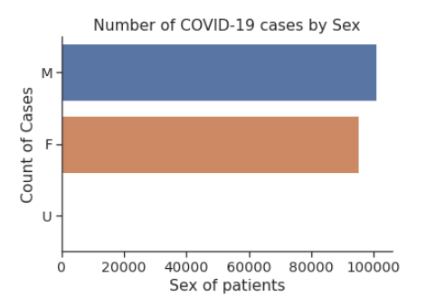
2.2: Counts of cases by Sex#
Using sns.countplot(), plot the number of all female and male cases.
Set the title to be “Number of COVID-19 cases by Sex”.
Hint: The documentation above contains some examples that might help you get started
Sample output#
# Your Solution here
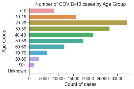
2.3: Counts of cases by Age Group#
Plot the counts of cases by age group, and order the y-axis by increasing age (use the order parameter of the countplot() function).
# Your Solution here
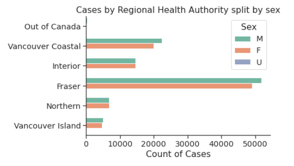
2.4: Cases by regional health authority#
Using set() data type, find the all the different regions in df['HA']. In the next step, print the set containing the different regions. Finally, using sns.countplot(), plot a horizontal bar chart of number of cases based on their regions.
Hint: Your plot doesn’t have to look exactly like this, but please do explore the possible color palettes. You can specify the colour palette by passing in the keyword like this: palette='colorblind'.
Sample output#
# Your solution here
2.5: Data Wrangling I#
Task: Add a new column to the dataframe to convert the “Reported_Date” column to a datetime object
To do this, first we need to add a new column to our dataset to turn the column “Reported_Date” into a proper datetime object so we can do operations on it.
Hint: Use to to_datetime() function to help you first convert it into a datetime object, and then remove the timezone information and HH:MM:SS using .dt.date.
# Your Solution here
2.6: Data Wrangling II#
Task: Find the earliest reported case and the latest reported case of COVID-19 in the dataset
You should use the pandas .min() and .max() functions here, now that your date string is converted to a DateTime object.
Sample Output#
The earliest reported case of COVID-19 was: 2020-01-29
The latest reported case of COVID-19 was: 2020-10-14
# Your Solution here
2.7: Data Wrangling III#
Task: Create a new column in the data frame called “days_since”.
This column will be of type integer, and will simply show the days since the first reported case of COVID-19.
Hint: Subtracting the earliest reported date from the Reported_Date_Object column will get you most of the way there. After that, the only thing left to is to turn the result (a datetime object) into an integer using .dt.days.
# Your Solution here
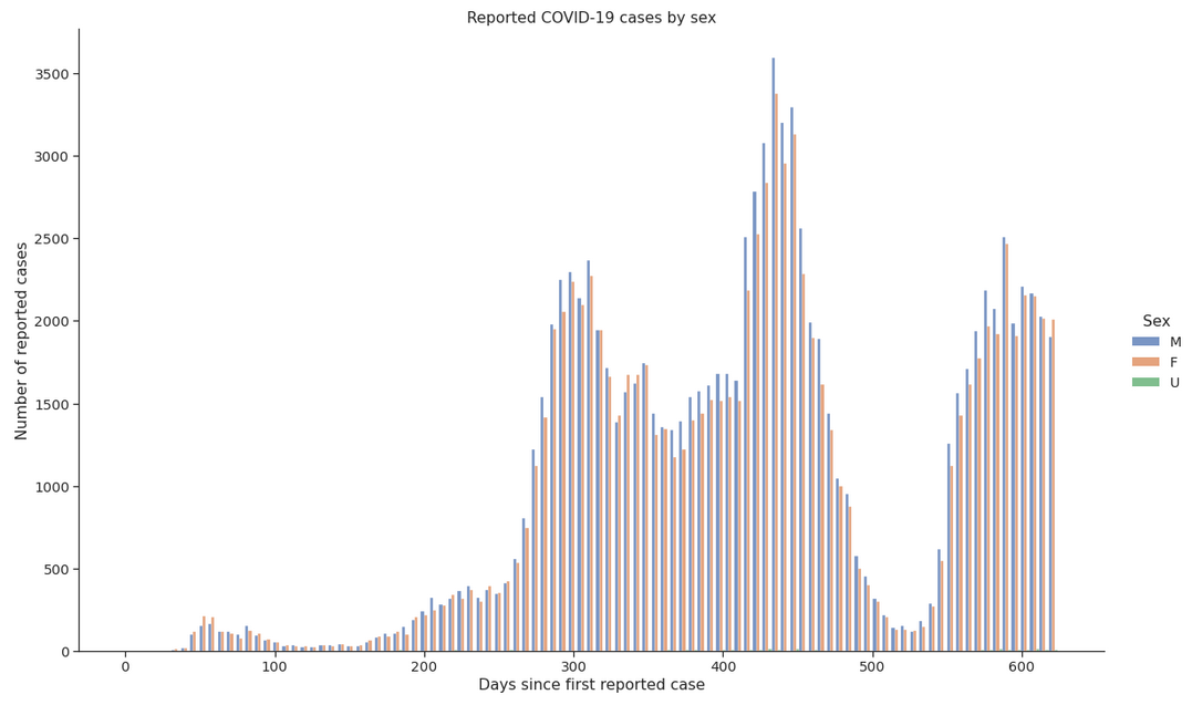
2.8: Plot the COVID-19 cases plotted over time by sex#
Using sns.displot, plot the histogram of females and males cases over time.
Hint 1: Here is a nice tutorial of all the different options that are possible when creating a histogram.
Sample output#
# Your Solution here
2.9: BONUS - For a bonus mark, move the legend to the top left of the plot#
Remember, the maximum mark you can get on a lab is 100% and bonus marks cannot be “moved” to different assignments”
# Your Solution here