Data Wrangling with Pandas II

Image by Hands off my tags! Michael Gaida from Pixabay.

Outline

In this class we will talk more about:

• “Tips and tricks” for working with pandas

• Handling Missing Data

• Combining Datasets: Concat and Append

• Visualizing Data using seaborn and pandas

• Additional Notes you may found helpful

Working with Pandas to load data

import pandas as pd

Always use RELATIVE paths!!

pwd

'/home/runner/work/data301_course/data301_course/notes/week05/Class5B'

!ls data/

chord-fingers1.csv  state-abbrevs.csv  state-population.csv
chord-fingers2.csv  state-areas.csv

What if your data is not UTF-8 encoded?

(Hint: You will get a UnicodeDecodeError)

url = "http://nfdp.ccfm.org/download/data/csv/NFD%20-%20Area%20burned%20by%20cause%20class%20-%20EN%20FR.csv"

dataset = pd.read_csv(url)

---------------------------------------------------------------------------
UnicodeDecodeError                        Traceback (most recent call last)
Cell In[4], line 3
      1 url = "http://nfdp.ccfm.org/download/data/csv/NFD%20-%20Area%20burned%20by%20cause%20class%20-%20EN%20FR.csv"
----> 3 dataset = pd.read_csv(url)

File /opt/hostedtoolcache/Python/3.10.9/x64/lib/python3.10/site-packages/pandas/util/_decorators.py:211, in deprecate_kwarg.<locals>._deprecate_kwarg.<locals>.wrapper(*args, **kwargs)
    209     else:
    210         kwargs[new_arg_name] = new_arg_value
--> 211 return func(*args, **kwargs)

File /opt/hostedtoolcache/Python/3.10.9/x64/lib/python3.10/site-packages/pandas/util/_decorators.py:331, in deprecate_nonkeyword_arguments.<locals>.decorate.<locals>.wrapper(*args, **kwargs)
    325 if len(args) > num_allow_args:
    326     warnings.warn(
    327         msg.format(arguments=_format_argument_list(allow_args)),
    328         FutureWarning,
    329         stacklevel=find_stack_level(),
    330     )
--> 331 return func(*args, **kwargs)

File /opt/hostedtoolcache/Python/3.10.9/x64/lib/python3.10/site-packages/pandas/io/parsers/readers.py:950, in read_csv(filepath_or_buffer, sep, delimiter, header, names, index_col, usecols, squeeze, prefix, mangle_dupe_cols, dtype, engine, converters, true_values, false_values, skipinitialspace, skiprows, skipfooter, nrows, na_values, keep_default_na, na_filter, verbose, skip_blank_lines, parse_dates, infer_datetime_format, keep_date_col, date_parser, dayfirst, cache_dates, iterator, chunksize, compression, thousands, decimal, lineterminator, quotechar, quoting, doublequote, escapechar, comment, encoding, encoding_errors, dialect, error_bad_lines, warn_bad_lines, on_bad_lines, delim_whitespace, low_memory, memory_map, float_precision, storage_options)
    935 kwds_defaults = _refine_defaults_read(
    936     dialect,
    937     delimiter,
   (...)
    946     defaults={"delimiter": ","},
    947 )
    948 kwds.update(kwds_defaults)
--> 950 return _read(filepath_or_buffer, kwds)

File /opt/hostedtoolcache/Python/3.10.9/x64/lib/python3.10/site-packages/pandas/io/parsers/readers.py:605, in _read(filepath_or_buffer, kwds)
    602 _validate_names(kwds.get("names", None))
    604 # Create the parser.
--> 605 parser = TextFileReader(filepath_or_buffer, **kwds)
    607 if chunksize or iterator:
    608     return parser

File /opt/hostedtoolcache/Python/3.10.9/x64/lib/python3.10/site-packages/pandas/io/parsers/readers.py:1442, in TextFileReader.__init__(self, f, engine, **kwds)
   1439     self.options["has_index_names"] = kwds["has_index_names"]
   1441 self.handles: IOHandles | None = None
-> 1442 self._engine = self._make_engine(f, self.engine)

File /opt/hostedtoolcache/Python/3.10.9/x64/lib/python3.10/site-packages/pandas/io/parsers/readers.py:1753, in TextFileReader._make_engine(self, f, engine)
   1750     raise ValueError(msg)
   1752 try:
-> 1753     return mapping[engine](f, **self.options)
   1754 except Exception:
   1755     if self.handles is not None:

File /opt/hostedtoolcache/Python/3.10.9/x64/lib/python3.10/site-packages/pandas/io/parsers/c_parser_wrapper.py:79, in CParserWrapper.__init__(self, src, **kwds)
     76     kwds.pop(key, None)
     78 kwds["dtype"] = ensure_dtype_objs(kwds.get("dtype", None))
---> 79 self._reader = parsers.TextReader(src, **kwds)
     81 self.unnamed_cols = self._reader.unnamed_cols
     83 # error: Cannot determine type of 'names'

File /opt/hostedtoolcache/Python/3.10.9/x64/lib/python3.10/site-packages/pandas/_libs/parsers.pyx:547, in pandas._libs.parsers.TextReader.__cinit__()

File /opt/hostedtoolcache/Python/3.10.9/x64/lib/python3.10/site-packages/pandas/_libs/parsers.pyx:636, in pandas._libs.parsers.TextReader._get_header()

File /opt/hostedtoolcache/Python/3.10.9/x64/lib/python3.10/site-packages/pandas/_libs/parsers.pyx:852, in pandas._libs.parsers.TextReader._tokenize_rows()

File /opt/hostedtoolcache/Python/3.10.9/x64/lib/python3.10/site-packages/pandas/_libs/parsers.pyx:1965, in pandas._libs.parsers.raise_parser_error()

UnicodeDecodeError: 'utf-8' codec can't decode byte 0xe9 in position 8: invalid continuation byte

Demo

Now what!?

Now we google it…

And according to this stack overflow page: we should try:

pd.read_csv(url, encoding='latin')

So let’s give it a shot:

pd.read_csv(url, encoding="latin")

# Works!!

	Year	Année	ISO	Jurisdiction	Juridiction	Cause	Origine	Area (hectares)	Data Qualifier	Superficie (en hectare)	Qualificatifs de données
0	1990	1990	AB	Alberta	Alberta	Human activity	Activités humaines	2393.8	a	2393.8	a
1	1990	1990	AB	Alberta	Alberta	Lightning	Foudre	55482.6	a	55482.6	a
2	1990	1990	AB	Alberta	Alberta	Unspecified	Indéterminée	1008.8	a	1008.8	a
3	1990	1990	BC	British Columbia	Colombie-Britannique	Human activity	Activités humaines	40278.3	a	40278.3	a
4	1990	1990	BC	British Columbia	Colombie-Britannique	Lightning	Foudre	35503.5	a	35503.5	a
...	...	...	...	...	...	...	...	...	...	...	...
1054	2021	2021	PC	Parks Canada	Parcs Canada	Unspecified	Indéterminée	42538.0	e	42538.0	e
1055	2021	2021	PE	Prince Edward Island	Île-du-Prince-Édouard	Unspecified	Indéterminée	0.1	e	0.1	e
1056	2021	2021	QC	Quebec	Québec	Unspecified	Indéterminée	49748.0	e	49748.0	e
1057	2021	2021	SK	Saskatchewan	Saskatchewan	Unspecified	Indéterminée	956084.0	e	956084.0	e
1058	2021	2021	YT	Yukon	Yukon	Unspecified	Indéterminée	118126.0	e	118126.0	e

1059 rows × 11 columns

What if your data is not comma-separated?

chord1 = pd.read_csv("data/chord-fingers1.csv")
chord1.head()

---------------------------------------------------------------------------
ParserError                               Traceback (most recent call last)
Input In [7], in <cell line: 1>()
----> 1 chord1 = pd.read_csv("data/chord-fingers1.csv")
      2 chord1.head()

File ~/.pyenv/versions/3.10.2/lib/python3.10/site-packages/pandas/util/_decorators.py:311, in deprecate_nonkeyword_arguments.<locals>.decorate.<locals>.wrapper(*args, **kwargs)
    305 if len(args) > num_allow_args:
    306     warnings.warn(
    307         msg.format(arguments=arguments),
    308         FutureWarning,
    309         stacklevel=stacklevel,
    310     )
--> 311 return func(*args, **kwargs)

File ~/.pyenv/versions/3.10.2/lib/python3.10/site-packages/pandas/io/parsers/readers.py:680, in read_csv(filepath_or_buffer, sep, delimiter, header, names, index_col, usecols, squeeze, prefix, mangle_dupe_cols, dtype, engine, converters, true_values, false_values, skipinitialspace, skiprows, skipfooter, nrows, na_values, keep_default_na, na_filter, verbose, skip_blank_lines, parse_dates, infer_datetime_format, keep_date_col, date_parser, dayfirst, cache_dates, iterator, chunksize, compression, thousands, decimal, lineterminator, quotechar, quoting, doublequote, escapechar, comment, encoding, encoding_errors, dialect, error_bad_lines, warn_bad_lines, on_bad_lines, delim_whitespace, low_memory, memory_map, float_precision, storage_options)
    665 kwds_defaults = _refine_defaults_read(
    666     dialect,
    667     delimiter,
   (...)
    676     defaults={"delimiter": ","},
    677 )
    678 kwds.update(kwds_defaults)
--> 680 return _read(filepath_or_buffer, kwds)

File ~/.pyenv/versions/3.10.2/lib/python3.10/site-packages/pandas/io/parsers/readers.py:581, in _read(filepath_or_buffer, kwds)
    578     return parser
    580 with parser:
--> 581     return parser.read(nrows)

File ~/.pyenv/versions/3.10.2/lib/python3.10/site-packages/pandas/io/parsers/readers.py:1254, in TextFileReader.read(self, nrows)
   1252 nrows = validate_integer("nrows", nrows)
   1253 try:
-> 1254     index, columns, col_dict = self._engine.read(nrows)
   1255 except Exception:
   1256     self.close()

File ~/.pyenv/versions/3.10.2/lib/python3.10/site-packages/pandas/io/parsers/c_parser_wrapper.py:225, in CParserWrapper.read(self, nrows)
    223 try:
    224     if self.low_memory:
--> 225         chunks = self._reader.read_low_memory(nrows)
    226         # destructive to chunks
    227         data = _concatenate_chunks(chunks)

File pandas/_libs/parsers.pyx:805, in pandas._libs.parsers.TextReader.read_low_memory()

File pandas/_libs/parsers.pyx:861, in pandas._libs.parsers.TextReader._read_rows()

File pandas/_libs/parsers.pyx:847, in pandas._libs.parsers.TextReader._tokenize_rows()

File pandas/_libs/parsers.pyx:1960, in pandas._libs.parsers.raise_parser_error()

ParserError: Error tokenizing data. C error: Expected 10 fields in line 7, saw 11

Demo

Now what!?

Now we google the error message…

And according to this stack overflow page: we should try:

pd.read_csv('data/chord-fingers1.csv', sep=';')

So let’s give it a shot:

chord1 = pd.read_csv("data/chord-fingers1.csv", sep=";")
chord1.head()

	CHORD_ROOT	CHORD_TYPE	CHORD_STRUCTURE	FINGER_POSITIONS	NOTE_NAMES
0	A#	13	1;3;5;b7;9;11;13	x,1,0,2,3,4	A#,C##,G#,B#,F##
1	A#	13	1;3;5;b7;9;11;13	4,x,3,2,1,1	A#,G#,B#,C##,F##
2	A#	13	1;3;5;b7;9;11;13	1,x,1,2,3,4	A#,G#,C##,F##,B#
3	A#	7(#9)	1;3;5;b7;#9	x,1,0,2,4,3	A#,C##,G#,B##,E#
4	A#	7(#9)	1;3;5;b7;#9	2,1,3,3,3,x	A#,C##,G#,B##,E#

# Let's load in the second part of the dataset in the same way:

chord2 = pd.read_csv("data/chord-fingers2.csv", sep=";")
chord2.head()

	CHORD_ROOT	CHORD_TYPE	CHORD_STRUCTURE	FINGER_POSITIONS	NOTE_NAMES
0	Ab	6	1;3;5;6	x,4,2,3,1,x	Ab,C,F,Ab
1	Ab	6	1;3;5;6	x,x,3,2,4,1	Ab,C,F,Ab
2	Ab	6	1;3;5;6	2,x,1,4,x,x	Ab,F,C
3	Ab	6	1;3;5;6	1,x,x,3,4,x	Ab,C,F
4	Ab	6	1;3;5;6	x,x,1,3,1,4	Ab,Eb,F,C

len(chord1)

598

len(chord2)

2034

len(chord1) + len(chord2)

2632

Combining DataFrames together

We saw that our dataset came in two parts (chord1 and chord2).

A common task in data analysis is to merge or combine datasets together. There are several combinations we can do.

Let’s look at just a basic one:

Using .concat()

Documentation on the .concat() function

# chord1['New Column'] ='Firas'
chord1

	CHORD_ROOT	CHORD_TYPE	CHORD_STRUCTURE	FINGER_POSITIONS	NOTE_NAMES
0	A#	13	1;3;5;b7;9;11;13	x,1,0,2,3,4	A#,C##,G#,B#,F##
1	A#	13	1;3;5;b7;9;11;13	4,x,3,2,1,1	A#,G#,B#,C##,F##
2	A#	13	1;3;5;b7;9;11;13	1,x,1,2,3,4	A#,G#,C##,F##,B#
3	A#	7(#9)	1;3;5;b7;#9	x,1,0,2,4,3	A#,C##,G#,B##,E#
4	A#	7(#9)	1;3;5;b7;#9	2,1,3,3,3,x	A#,C##,G#,B##,E#
...	...	...	...	...	...
593	Ab	m7	1;b3;5;b7	1,3,1,1,1,x	Ab,Eb,Gb,Cb,Eb
594	Ab	dim	1;b3;b5	x,x,4,3,1,2	Ab,Cb,Ebb,Ab
595	Ab	dim	1;b3;b5	x,1,2,4,3,x	Ab,Ebb,Ab,Cb
596	Ab	6	1;3;5;6	x,x,1,1,1,1	Eb,Ab,C,F
597	Ab	6	1;3;5;6	1,x,3,2,4,1	Ab,Ab,C,F,Ab

598 rows × 5 columns

pd.concat([chord1, chord2])

	CHORD_ROOT	CHORD_TYPE	CHORD_STRUCTURE	FINGER_POSITIONS	NOTE_NAMES	New Column
0	A#	13	1;3;5;b7;9;11;13	x,1,0,2,3,4	A#,C##,G#,B#,F##	Firas
1	A#	13	1;3;5;b7;9;11;13	4,x,3,2,1,1	A#,G#,B#,C##,F##	Firas
2	A#	13	1;3;5;b7;9;11;13	1,x,1,2,3,4	A#,G#,C##,F##,B#	Firas
3	A#	7(#9)	1;3;5;b7;#9	x,1,0,2,4,3	A#,C##,G#,B##,E#	Firas
4	A#	7(#9)	1;3;5;b7;#9	2,1,3,3,3,x	A#,C##,G#,B##,E#	Firas
...	...	...	...	...	...	...
2029	G	sus4	1;4;5	x,1,2,3,4,1	G,D,G,C,D	NaN
2030	G	sus4	1;4;5	x,x,3,4,1,1	G,C,D,G	NaN
2031	G	6/9	1;3;5;6;9	2,1,1,1,3,4	G,B,E,A,D,G	NaN
2032	G	6/9	1;3;5;6;9	x,x,2,1,3,4	G,B,E,A	NaN
2033	G	6/9	1;3;5;6;9	x,2,1,1,3,4	G,B,E,A,D	NaN

2632 rows × 6 columns

# You NEED to save the output of all pandas function, do NOT use the "inplace" argument, it will be deprecated soon

chords = pd.concat([chord1, chord2])

chords

	CHORD_ROOT	CHORD_TYPE	CHORD_STRUCTURE	FINGER_POSITIONS	NOTE_NAMES
0	A#	13	1;3;5;b7;9;11;13	x,1,0,2,3,4	A#,C##,G#,B#,F##
1	A#	13	1;3;5;b7;9;11;13	4,x,3,2,1,1	A#,G#,B#,C##,F##
2	A#	13	1;3;5;b7;9;11;13	1,x,1,2,3,4	A#,G#,C##,F##,B#
3	A#	7(#9)	1;3;5;b7;#9	x,1,0,2,4,3	A#,C##,G#,B##,E#
4	A#	7(#9)	1;3;5;b7;#9	2,1,3,3,3,x	A#,C##,G#,B##,E#
...	...	...	...	...	...
2029	G	sus4	1;4;5	x,1,2,3,4,1	G,D,G,C,D
2030	G	sus4	1;4;5	x,x,3,4,1,1	G,C,D,G
2031	G	6/9	1;3;5;6;9	2,1,1,1,3,4	G,B,E,A,D,G
2032	G	6/9	1;3;5;6;9	x,x,2,1,3,4	G,B,E,A
2033	G	6/9	1;3;5;6;9	x,2,1,1,3,4	G,B,E,A,D

2632 rows × 5 columns

Using .rename()

Documentation on the .rename() function:

# Capitals annoy me!

list(chords.columns)

['CHORD_ROOT',
 'CHORD_TYPE',
 'CHORD_STRUCTURE',
 'FINGER_POSITIONS',
 'NOTE_NAMES']

chords = chords.rename(
     
)
chords.head() 

	Chord	Type	Structure	Finger	Notes
0	A#	13	1;3;5;b7;9;11;13	x,1,0,2,3,4	A#,C##,G#,B#,F##
1	A#	13	1;3;5;b7;9;11;13	4,x,3,2,1,1	A#,G#,B#,C##,F##
2	A#	13	1;3;5;b7;9;11;13	1,x,1,2,3,4	A#,G#,C##,F##,B#
3	A#	7(#9)	1;3;5;b7;#9	x,1,0,2,4,3	A#,C##,G#,B##,E#
4	A#	7(#9)	1;3;5;b7;#9	2,1,3,3,3,x	A#,C##,G#,B##,E#

Using .replace()

Documentation on the .replace() function:

chords_cleaned = chords.replace("A#", "A-sharp")
chords_cleaned

	Chord	Type	Structure	Finger	Notes
0	A-sharp	13	1;3;5;b7;9;11;13	x,1,0,2,3,4	A#,C##,G#,B#,F##
1	A-sharp	13	1;3;5;b7;9;11;13	4,x,3,2,1,1	A#,G#,B#,C##,F##
2	A-sharp	13	1;3;5;b7;9;11;13	1,x,1,2,3,4	A#,G#,C##,F##,B#
3	A-sharp	7(#9)	1;3;5;b7;#9	x,1,0,2,4,3	A#,C##,G#,B##,E#
4	A-sharp	7(#9)	1;3;5;b7;#9	2,1,3,3,3,x	A#,C##,G#,B##,E#
...	...	...	...	...	...
2029	G	sus4	1;4;5	x,1,2,3,4,1	G,D,G,C,D
2030	G	sus4	1;4;5	x,x,3,4,1,1	G,C,D,G
2031	G	6/9	1;3;5;6;9	2,1,1,1,3,4	G,B,E,A,D,G
2032	G	6/9	1;3;5;6;9	x,x,2,1,3,4	G,B,E,A
2033	G	6/9	1;3;5;6;9	x,2,1,1,3,4	G,B,E,A,D

2632 rows × 5 columns

Using .drop()

Documentation on the .drop() function:

chords_cleaned

	Chord	Type	Structure	Finger	Notes
0	A-sharp	13	1;3;5;b7;9;11;13	x,1,0,2,3,4	A#,C##,G#,B#,F##
1	A-sharp	13	1;3;5;b7;9;11;13	4,x,3,2,1,1	A#,G#,B#,C##,F##
2	A-sharp	13	1;3;5;b7;9;11;13	1,x,1,2,3,4	A#,G#,C##,F##,B#
3	A-sharp	7(#9)	1;3;5;b7;#9	x,1,0,2,4,3	A#,C##,G#,B##,E#
4	A-sharp	7(#9)	1;3;5;b7;#9	2,1,3,3,3,x	A#,C##,G#,B##,E#
...	...	...	...	...	...
2029	G	sus4	1;4;5	x,1,2,3,4,1	G,D,G,C,D
2030	G	sus4	1;4;5	x,x,3,4,1,1	G,C,D,G
2031	G	6/9	1;3;5;6;9	2,1,1,1,3,4	G,B,E,A,D,G
2032	G	6/9	1;3;5;6;9	x,x,2,1,3,4	G,B,E,A
2033	G	6/9	1;3;5;6;9	x,2,1,1,3,4	G,B,E,A,D

2632 rows × 5 columns

chords_cleaned = chords_cleaned.drop(["Notes", "New Column"], axis="columns")

sorted(list(chords_cleaned.columns))

['Chord', 'Finger', 'Structure', 'Type']

chords = chords[sorted(list(chords.columns))]

chords

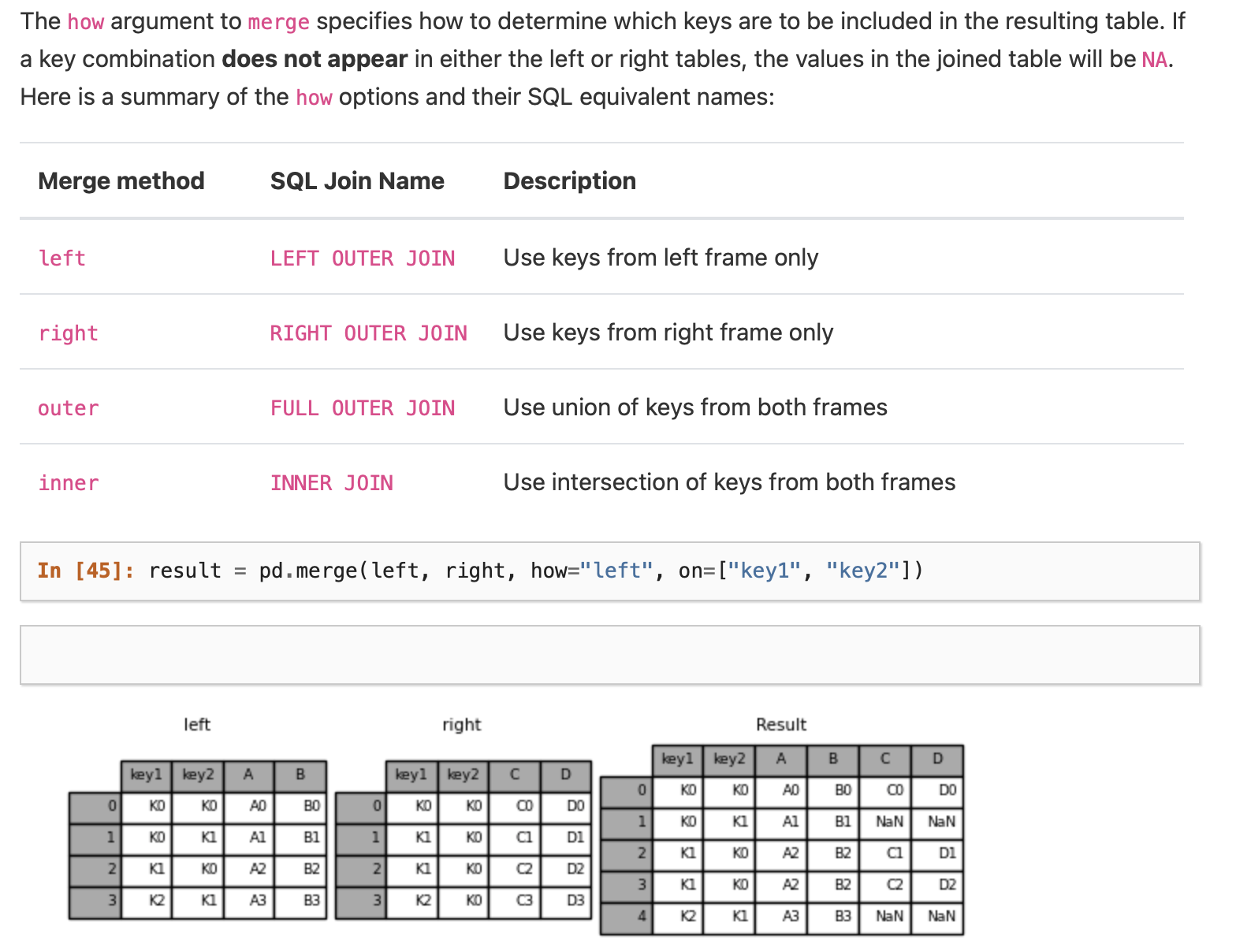
Using .merge()

User Guide on Merging Dataframes on the .merge() function

Visualizing Data using seaborn and pandas

This is a preview of content coming later!

# You may need to install seaborn:
# Remember the command to install a package `conda install -c conda-forge seaborn`

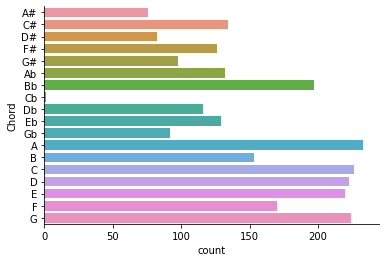
import seaborn as sns

sns.countplot(y="Chord", data=chords)
sns.despine()

Additional Notes on Handling Missing Data

Attribution

This notebook contains an excerpt from the Python Data Science Handbook by Jake VanderPlas; the content is available on GitHub.

The text is released under the CC-BY-NC-ND license, and code is released under the MIT license. If you find this content useful, please consider supporting the work by buying the book!

The difference between data found in many tutorials and data in the real world is that real-world data is rarely clean and homogeneous. In particular, many interesting datasets will have some amount of data missing. To make matters even more complicated, different data sources may indicate missing data in different ways.

In this section, we will discuss some general considerations for missing data, discuss how Pandas chooses to represent it, and demonstrate some built-in Pandas tools for handling missing data in Python. Here and throughout the book, we’ll refer to missing data in general as null, NaN, or NA values.

Trade-Offs in Missing Data Conventions

There are a number of schemes that have been developed to indicate the presence of missing data in a table or DataFrame. Generally, they revolve around one of two strategies: using a mask that globally indicates missing values, or choosing a sentinel value that indicates a missing entry.

In the masking approach, the mask might be an entirely separate Boolean array, or it may involve appropriation of one bit in the data representation to locally indicate the null status of a value.

In the sentinel approach, the sentinel value could be some data-specific convention, such as indicating a missing integer value with -9999 or some rare bit pattern, or it could be a more global convention, such as indicating a missing floating-point value with NaN (Not a Number), a special value which is part of the IEEE floating-point specification.

None of these approaches is without trade-offs: use of a separate mask array requires allocation of an additional Boolean array, which adds overhead in both storage and computation. A sentinel value reduces the range of valid values that can be represented, and may require extra (often non-optimized) logic in CPU and GPU arithmetic. Common special values like NaN are not available for all data types.

As in most cases where no universally optimal choice exists, different languages and systems use different conventions. For example, the R language uses reserved bit patterns within each data type as sentinel values indicating missing data, while the SciDB system uses an extra byte attached to every cell which indicates a NA state.

Missing Data in Pandas

The way in which Pandas handles missing values is constrained by its reliance on the NumPy package, which does not have a built-in notion of NA values for non-floating-point data types.

Pandas could have followed R’s lead in specifying bit patterns for each individual data type to indicate nullness, but this approach turns out to be rather unwieldy. While R contains four basic data types, NumPy supports far more than this: for example, while R has a single integer type, NumPy supports fourteen basic integer types once you account for available precisions, signedness, and endianness of the encoding. Reserving a specific bit pattern in all available NumPy types would lead to an unwieldy amount of overhead in special-casing various operations for various types, likely even requiring a new fork of the NumPy package. Further, for the smaller data types (such as 8-bit integers), sacrificing a bit to use as a mask will significantly reduce the range of values it can represent.

NumPy does have support for masked arrays – that is, arrays that have a separate Boolean mask array attached for marking data as “good” or “bad.” Pandas could have derived from this, but the overhead in both storage, computation, and code maintenance makes that an unattractive choice.

With these constraints in mind, Pandas chose to use sentinels for missing data, and further chose to use two already-existing Python null values: the special floating-point NaN value, and the Python None object. This choice has some side effects, as we will see, but in practice ends up being a good compromise in most cases of interest.

None: Pythonic missing data

The first sentinel value used by Pandas is None, a Python singleton object that is often used for missing data in Python code. Because it is a Python object, None cannot be used in any arbitrary NumPy/Pandas array, but only in arrays with data type 'object' (i.e., arrays of Python objects):

import numpy as np
import pandas as pd

vals1 = np.array([1, None, 3, 4])
vals1

This dtype=object means that the best common type representation NumPy could infer for the contents of the array is that they are Python objects. While this kind of object array is useful for some purposes, any operations on the data will be done at the Python level, with much more overhead than the typically fast operations seen for arrays with native types:

for dtype in ["object", "int"]:
    print("dtype =", dtype)
    %timeit np.arange(1E6, dtype=dtype).sum()
    print()

The use of Python objects in an array also means that if you perform aggregations like sum() or min() across an array with a None value, you will generally get an error:

vals1

1 + None

vals1.sum()

This reflects the fact that addition between an integer and None is undefined.

NaN: Missing numerical data

The other missing data representation, NaN (acronym for Not a Number), is different; it is a special floating-point value recognized by all systems that use the standard IEEE floating-point representation:

vals2 = np.array([1, np.nan, 3, 4])
vals2.dtype

Notice that NumPy chose a native floating-point type for this array: this means that unlike the object array from before, this array supports fast operations pushed into compiled code. You should be aware that NaN is a bit like a data virus–it infects any other object it touches. Regardless of the operation, the result of arithmetic with NaN will be another NaN:

1 + np.nan

0 * np.nan

Note that this means that aggregates over the values are well defined (i.e., they don’t result in an error) but not always useful:

vals2.sum(), vals2.min(), vals2.max()

NumPy does provide some special aggregations that will ignore these missing values:

np.nansum(vals2), np.nanmin(vals2), np.nanmax(vals2)

Keep in mind that NaN is specifically a floating-point value; there is no equivalent NaN value for integers, strings, or other types.

NaN and None in Pandas

NaN and None both have their place, and Pandas is built to handle the two of them nearly interchangeably, converting between them where appropriate:

pd.Series([1, np.nan, 2, None])

For types that don’t have an available sentinel value, Pandas automatically type-casts when NA values are present. For example, if we set a value in an integer array to np.nan, it will automatically be upcast to a floating-point type to accommodate the NA:

x = pd.Series(range(2), dtype=int)
x

x[0] = None
x

Notice that in addition to casting the integer array to floating point, Pandas automatically converts the None to a NaN value. (Be aware that there is a proposal to add a native integer NA to Pandas in the future; as of this writing, it has not been included).

While this type of magic may feel a bit hackish compared to the more unified approach to NA values in domain-specific languages like R, the Pandas sentinel/casting approach works quite well in practice and in my experience only rarely causes issues.

The following table lists the upcasting conventions in Pandas when NA values are introduced:

Typeclass	Conversion When Storing NAs	NA Sentinel Value
floating	No change	np.nan
object	No change	None or np.nan
integer	Cast to float64	np.nan
boolean	Cast to object	None or np.nan

Keep in mind that in Pandas, string data is always stored with an object dtype.

Operating on Null Values

As we have seen, Pandas treats None and NaN as essentially interchangeable for indicating missing or null values. To facilitate this convention, there are several useful methods for detecting, removing, and replacing null values in Pandas data structures. They are:

• isnull(): Generate a boolean mask indicating missing values

• notnull(): Opposite of isnull()

• dropna(): Return a filtered version of the data

• fillna(): Return a copy of the data with missing values filled or imputed

We will conclude this section with a brief exploration and demonstration of these routines.

Detecting null values

Pandas data structures have two useful methods for detecting null data: isnull() and notnull(). Either one will return a Boolean mask over the data. For example:

data = pd.DataFrame([1, np.nan, "hello", None])
data

data[data.notnull()]

data.isnull()

As mentioned in Data Indexing and Selection, Boolean masks can be used directly as a Series or DataFrame index:

data[data.notnull()]

The isnull() and notnull() methods produce similar Boolean results for DataFrames.

Dropping null values

In addition to the masking used before, there are the convenience methods, dropna() (which removes NA values) and fillna() (which fills in NA values). For a Series, the result is straightforward:

data

data.dropna().reset_index(drop=True)

For a DataFrame, there are more options. Consider the following DataFrame:

df = pd.DataFrame([[1, np.nan, 2], [2, 3, 5], [np.nan, 4, 6]])
df

We cannot drop single values from a DataFrame; we can only drop full rows or full columns. Depending on the application, you might want one or the other, so dropna() gives a number of options for a DataFrame.

By default, dropna() will drop all rows in which any null value is present:

df.dropna()

Alternatively, you can drop NA values along a different axis; axis=1 drops all columns containing a null value:

df.dropna(axis="columns")

But this drops some good data as well; you might rather be interested in dropping rows or columns with all NA values, or a majority of NA values. This can be specified through the how or thresh parameters, which allow fine control of the number of nulls to allow through.

The default is how='any', such that any row or column (depending on the axis keyword) containing a null value will be dropped. You can also specify how='all', which will only drop rows/columns that are all null values:

df[3] = np.nan
df

df.dropna(axis="columns", how="all")

For finer-grained control, the thresh parameter lets you specify a minimum number of non-null values for the row/column to be kept:

df.dropna(axis="rows", thresh=3)

Here the first and last row have been dropped, because they contain only two non-null values.

Filling null values

Sometimes rather than dropping NA values, you’d rather replace them with a valid value. This value might be a single number like zero, or it might be some sort of imputation or interpolation from the good values. You could do this in-place using the isnull() method as a mask, but because it is such a common operation Pandas provides the fillna() method, which returns a copy of the array with the null values replaced.

Consider the following Series:

data = pd.Series([1, np.nan, 2, None, 3], index=list("abcde"))
data

np.mean(data)

We can fill NA entries with a single value, such as zero:

data.fillna(0)

data.fillna(0).mean()

We can specify a forward-fill to propagate the previous value forward:

# forward-fill
data.fillna(method="ffill")

Or we can specify a back-fill to propagate the next values backward:

# back-fill
data.fillna(method="bfill")

For DataFrames, the options are similar, but we can also specify an axis along which the fills take place:

df

df.fillna(method="ffill", axis="columns")

Notice that if a previous value is not available during a forward fill, the NA value remains.

Combining Datasets: Concat and Append

Some of the most interesting studies of data come from combining different data sources. These operations can involve anything from very straightforward concatenation of two different datasets, to more complicated database-style joins and merges that correctly handle any overlaps between the datasets. Series and DataFrames are built with this type of operation in mind, and Pandas includes functions and methods that make this sort of data wrangling fast and straightforward.

Here we’ll take a look at simple concatenation of Series and DataFrames with the pd.concat function; later we’ll dive into more sophisticated in-memory merges and joins implemented in Pandas.

We begin with the standard imports:

import pandas as pd
import numpy as np

For convenience, we’ll define this function which creates a DataFrame of a particular form that will be useful below:

def make_df(cols, ind):
    """Quickly make a DataFrame"""
    data = {c: [str(c) + str(i) for i in ind] for c in cols}
    return pd.DataFrame(data, ind)


# example DataFrame
make_df("ABC", range(3))

In addition, we’ll create a quick class that allows us to display multiple DataFrames side by side. The code makes use of the special _repr_html_ method, which IPython uses to implement its rich object display:

class display(object):
    """Display HTML representation of multiple objects"""

    template = """<div style="float: left; padding: 10px;">
    <p style='font-family:"Courier New", Courier, monospace'>{0}</p>{1}
    </div>"""

    def __init__(self, *args):
        self.args = args

    def _repr_html_(self):
        return "\n".join(
            self.template.format(a, eval(a)._repr_html_()) for a in self.args
        )

    def __repr__(self):
        return "\n\n".join(a + "\n" + repr(eval(a)) for a in self.args)

The use of this will become clearer as we continue our discussion in the following section.

Recall: Concatenation of NumPy Arrays

Concatenation of Series and DataFrame objects is very similar to concatenation of Numpy arrays, which can be done via the np.concatenate function as discussed in The Basics of NumPy Arrays. Recall that with it, you can combine the contents of two or more arrays into a single array:

x = [1, 2, 3]
y = [4, 5, 6]
z = [7, 8, 9]
np.concatenate([x, y, z])

The first argument is a list or tuple of arrays to concatenate. Additionally, it takes an axis keyword that allows you to specify the axis along which the result will be concatenated:

x = [[1, 2], [3, 4]]
np.concatenate([x, x], axis=1)

Simple Concatenation with pd.concat

Pandas has a function, pd.concat(), which has a similar syntax to np.concatenate but contains a number of options that we’ll discuss momentarily:

# Signature in Pandas v0.18
pd.concat(objs, axis=0, join='outer', join_axes=None, ignore_index=False,
          keys=None, levels=None, names=None, verify_integrity=False,
          copy=True)

pd.concat() can be used for a simple concatenation of Series or DataFrame objects, just as np.concatenate() can be used for simple concatenations of arrays:

ser1 = pd.Series(["A", "B", "C"], index=[1, 2, 3])
ser2 = pd.Series(["D", "E", "F"], index=[4, 5, 6])
pd.concat([ser1, ser2])

It also works to concatenate higher-dimensional objects, such as DataFrames:

df1 = make_df("AB", [1, 2])
df2 = make_df("AB", [3, 4])
display("df1", "df2", "pd.concat([df1, df2])")

By default, the concatenation takes place row-wise within the DataFrame (i.e., axis='rows'). Like np.concatenate, pd.concat allows specification of an axis along which concatenation will take place. Consider the following example:

df3 = make_df("AB", [0, 1])
df4 = make_df("CD", [0, 1])
display("df3", "df4", "pd.concat([df3, df4], axis='col')")

We could have equivalently specified axis=1; here we’ve used the more intuitive axis='col'.

Duplicate indices

One important difference between np.concatenate and pd.concat is that Pandas concatenation preserves indices, even if the result will have duplicate indices! Consider this simple example:

x = make_df("AB", [0, 1])
y = make_df("AB", [2, 3])
y.index = x.index  # make duplicate indices!
display("x", "y", "pd.concat([x, y])")

Notice the repeated indices in the result. While this is valid within DataFrames, the outcome is often undesirable. pd.concat() gives us a few ways to handle it.

Catching the repeats as an error

If you’d like to simply verify that the indices in the result of pd.concat() do not overlap, you can specify the verify_integrity flag. With this set to True, the concatenation will raise an exception if there are duplicate indices. Here is an example, where for clarity we’ll catch and print the error message:

pd.concat([x, y])

try:
    pd.concat([x, y], verify_integrity=True)
except ValueError as e:
    print("ValueError:", e)

Ignoring the index

Sometimes the index itself does not matter, and you would prefer it to simply be ignored. This option can be specified using the ignore_index flag. With this set to true, the concatenation will create a new integer index for the resulting Series:

display("x", "y", "pd.concat([x, y], ignore_index=True)")

Adding MultiIndex keys

Another option is to use the keys option to specify a label for the data sources; the result will be a hierarchically indexed series containing the data:

display("x", "y", "pd.concat([x, y], keys=['x', 'y'])")

The result is a multiply indexed DataFrame, and we can use the tools discussed in Hierarchical Indexing to transform this data into the representation we’re interested in.

Concatenation with joins

In the simple examples we just looked at, we were mainly concatenating DataFrames with shared column names. In practice, data from different sources might have different sets of column names, and pd.concat offers several options in this case. Consider the concatenation of the following two DataFrames, which have some (but not all!) columns in common:

df5 = make_df("ABC", [1, 2])
df6 = make_df("BCD", [3, 4])
display("df5", "df6", "pd.concat([df5, df6])")

By default, the entries for which no data is available are filled with NA values. To change this, we can specify one of several options for the join and join_axes parameters of the concatenate function. By default, the join is a union of the input columns (join='outer'), but we can change this to an intersection of the columns using join='inner':

display("df5", "df6", "pd.concat([df5, df6], join='inner')")

Another option is to directly specify the index of the remaininig colums using the join_axes argument, which takes a list of index objects. Here we’ll specify that the returned columns should be the same as those of the first input:

display(‘df5’, ‘df6’, “pd.concat([df5, df6], join_axes=[df5.columns])”)

The combination of options of the pd.concat function allows a wide range of possible behaviors when joining two datasets; keep these in mind as you use these tools for your own data.

The append() method

Because direct array concatenation is so common, Series and DataFrame objects have an append method that can accomplish the same thing in fewer keystrokes. For example, rather than calling pd.concat([df1, df2]), you can simply call df1.append(df2):

display("df1", "df2", "df1.append(df2)")

Keep in mind that unlike the append() and extend() methods of Python lists, the append() method in Pandas does not modify the original object–instead it creates a new object with the combined data. It also is not a very efficient method, because it involves creation of a new index and data buffer. Thus, if you plan to do multiple append operations, it is generally better to build a list of DataFrames and pass them all at once to the concat() function.

In the next section, we’ll look at another more powerful approach to combining data from multiple sources, the database-style merges/joins implemented in pd.merge. For more information on concat(), append(), and related functionality, see the “Merge, Join, and Concatenate” section of the Pandas documentation.