Data Wrangling with Pandas I#

Image by Hands off my tags! Michael Gaida from Pixabay.

Outline#

In this lecture we will talk about:

How to do Data Analysis
Installing and Using Pandas
Data Manipulation with Pandas
Introducing DataFrames
Creating a DataFrame
Operating on Data in Pandas

How to do Data Analysis#

Here are some common steps of an analysis pipeline (the order isn’t set, and not all elements are necessary):

Load Data
- Check file types and encodings.
- Check delimiters (space, comma, tab).
- Skip rows and columns as needed.

Clean Data
- Remove columns not being used.
- Deal with “incorrect” data.
- Deal with missing data.

Process Data
- Create any new columns needed that are combinations or aggregates of other columns (examples include weighted averages, categorizations, groups, etc…).
- Find and replace operations (examples inlcude replacing the string ‘Strongly Agree’ with the number 5).
- Other substitutions as needed.
- Deal with outliers.

Wrangle Data
- Restructure data format (columns and rows).
- Merge other data sources into your dataset.

Exploratory Data Analysis
- More about thisafter the last class of the week

Data Analysis (not required until Milestone 3).
- In this course we will some data analysis, but the possibilities are endless here!

Export reports/data analyses and visualizations.

Data Manipulation with Pandas#

Attribution#

This notebook contains an excerpt from the Python Data Science Handbook by Jake VanderPlas; the content is available on GitHub.

The text is released under the CC-BY-NC-ND license, and code is released under the MIT license. If you find this content useful, please consider supporting the work by buying the book!

In this chapter, we will be looking in detail at the data structures provided by the Pandas library. Pandas is a newer package built on top of NumPy, and provides an efficient implementation of a DataFrame. DataFrames are essentially multidimensional arrays with attached row and column labels, and often with heterogeneous types and/or missing data. As well as offering a convenient storage interface for labeled data, Pandas implements a number of powerful data operations familiar to users of both database frameworks and spreadsheet programs.

NumPy’s ndarray data structure provides essential features for the type of clean, well-organized data typically seen in numerical computing tasks. While it serves this purpose very well, its limitations become clear when we need more flexibility (e.g., attaching labels to data, working with missing data, etc.) and when attempting operations that do not map well to element-wise broadcasting (e.g., groupings, pivots, etc.), each of which is an important piece of analyzing the less structured data available in many forms in the world around us. Pandas, and in particular its DataFrame object, building on the NumPy array structure and provides efficient access to these sorts of “data munging” tasks that occupy much of a data scientist’s time.

In this chapter, we will focus on the mechanics of using the DataFrame and related structures effectively. We will use examples drawn from real datasets where appropriate, but these examples are not necessarily the focus.

Installing and Using Pandas#

Installation of Pandas on your system requires NumPy to be installed, and if building the library from source, requires the appropriate tools to compile the C and Cython sources on which Pandas is built. Details on this installation can be found in the Pandas documentation.

To install pandas, open up a Terminal and install it using conda:

conda install pandas

Just as we generally import NumPy under the alias np, we will import Pandas under the alias pd:

import numpy as np
import pandas as pd 

This import convention will be used throughout the remainder of this book.

Once Pandas is installed, and imported you can check the version:

pd.__version__

'1.5.2'

Reminder about Built-In Documentation#

As you read through this chapter, don’t forget that IPython gives you the ability to quickly explore the contents of a package (by using the tab-completion feature) as well as the documentation of various functions (using the ? character). (Refer back to Help and Documentation in IPython if you need a refresher on this.)

For example, to display all the contents of the pandas namespace, you can type

In [3]: pd.<TAB>

And to display Pandas’s built-in documentation, you can use this:

In [4]: pd?

More detailed documentation, along with tutorials and other resources, can be found at http://pandas.pydata.org/.

Introducing DataFrames#

At the very basic level, Pandas objects can be thought of as enhanced versions of NumPy structured arrays in which the rows and columns are identified with labels rather than simple integer indices. As we will see during the course of this chapter, Pandas provides a host of useful tools, methods, and functionality on top of the basic data structures, but nearly everything that follows will require an understanding of what these structures are. Thus, before we go any further, let’s introduce these three fundamental Pandas data structures: the Series, DataFrame, and Index.

We will start our code sessions with the standard NumPy and Pandas imports:

import numpy as np
import pandas as pd

The fundamental structure in Pandas is the DataFrame. Like the Series object discussed in the previous section, the DataFrame can be thought of either as a generalization of a NumPy array, or as a specialization of a Python dictionary. We’ll now take a look at each of these perspectives.

Creating a DataFrame#

There are several ways of creating DataFrames in Python using Pandas and though it can end up with the same end product, the method of creating them can depend on the format of your data.

Let’s look at a few examples:

DataFrame from URL#

If your dataset exists on the web as a publicly accessible file, you can create a DataFrame directly from the URL to the CSV.

read_csv(path) is a function from the Pandas package that creates a DataFrame from a CSV file.
- The argument path can be a URL or a reference to a local file.

pd.read_csv("https://github.com/firasm/bits/raw/master/fruits.csv")

	Fruit Name	Mass(g)	Colour	Rating
0	Apple	200	Red	8
1	Banana	250	Yellow	9
2	Cantoloupe	600	Orange	10

I can store the dataframe as an object like this:

fruits = pd.read_csv("https://github.com/firasm/bits/raw/master/fruits.csv")

fruits

	Fruit Name	Mass(g)	Colour	Rating
0	Apple	200	Red	8
1	Banana	250	Yellow	9
2	Cantoloupe	600	Orange	10

You can print the first 5 lines of the dataset using the head() function (this data set only has 3 lines):

fruits.head()

	Fruit Name	Mass(g)	Colour	Rating
0	Apple	200	Red	8
1	Banana	250	Yellow	9
2	Cantoloupe	600	Orange	10

fruits["Colour"]

     Red
  Yellow
  Orange
Name: Colour, dtype: object

fruits["Rating"]

   8
   9
  10
Name: Rating, dtype: int64

fruits["Fruit Name"]

       Apple
      Banana
  Cantoloupe
Name: Fruit Name, dtype: object

fruits["Rating"].sum()

DataFrame from List of Dictionaries#

fruit1 = {"Fruit Name": "Apple", "Mass(g)": 200, "Colour": "Red", "Rating": 8}

fruit2 = {"Fruit Name": "Banana", "Mass(g)": 250, "Colour": "Yellow", "Rating": 9}

fruit3 = {"Fruit Name": "Cantoloupe", "Mass(g)": 600, "Colour": "Orange", "Rating": 10}

pd.DataFrame([fruit1, fruit2, fruit3])

	Fruit Name	Mass(g)	Colour	Rating
0	Apple	200	Red	8
1	Banana	250	Yellow	9
2	Cantoloupe	600	Orange	10

DataFrame from List of Tuples#

fruit_tuples = [
    ("Apple", "Red", 200, 8),
    ("Banana", 250, "Yellow", 9),
    ("Cantoloupe", 600, "Orange", 10),
]

labels = ["Fruit Name", "Mass(g)", "Color", "Rating"]

pd.DataFrame(fruit_tuples, columns=labels)

	Fruit Name	Mass(g)	Color	Rating
0	Apple	Red	200	8
1	Banana	250	Yellow	9
2	Cantoloupe	600	Orange	10

DataFrame from a Dictionary#

fruit_dict = {
    "Fruit Name": {0: "Apple", 1: "Banana", 2: "Cantoloupe"},
    "Mass(g)": {0: 200, 1: 250, 2: 600},
    "Colour": {0: "Red", 1: "Yellow", 2: "Orange"},
    "Rating": {0: 8, 1: 9, 2: 10},
}

pd.DataFrame.from_dict(fruit_dict)

	Fruit Name	Mass(g)	Colour	Rating
0	Apple	200	Red	8
1	Banana	250	Yellow	9
2	Cantoloupe	600	Orange	10

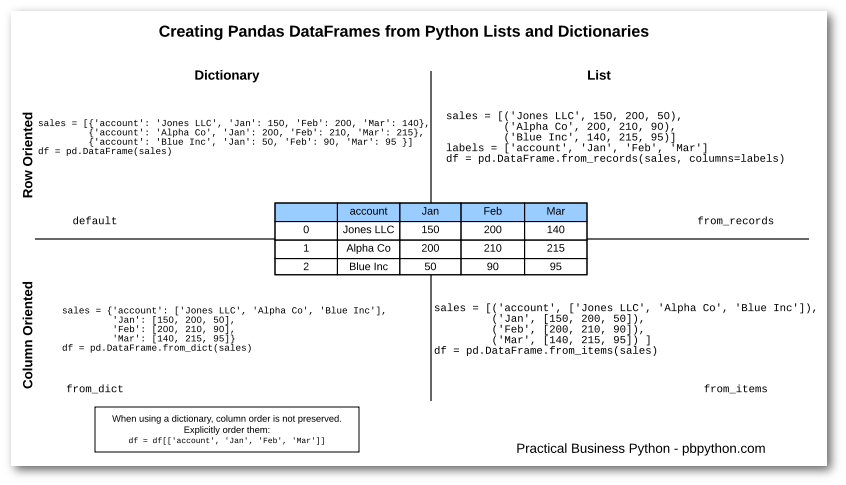
Here’s a great cheat sheet from “Practical Business Python (PBP)”:

https://pbpython.com/images/pandas-dataframe-shadow.png

Additionally, the DataFrame has a columns attribute, which is an Index object holding the column labels:

list(fruits.columns)

['Fruit Name', 'Mass(g)', 'Colour', 'Rating']

Thus the DataFrame can be thought of as a generalization of a two-dimensional NumPy array, where both the rows and columns have a generalized index for accessing the data.

Other ways of creating a DataFrame#

From a list of dicts#

Any list of dictionaries can be made into a DataFrame. We’ll use a simple list comprehension to create some data:

data = [{"a": i, "b": 2 * i} for i in range(3)]  # list comprehension!

pd.DataFrame(data)

	a	b
0	0	0
1	1	2
2	2	4

Even if some keys in the dictionary are missing, Pandas will fill them in with NaN (i.e., “not a number”) values:

pd.DataFrame([{"a": 1, "b": 2}, {"b": 3, "c": 4}])

	a	b	c
0	1.0	2	NaN
1	NaN	3	4.0

From a two-dimensional NumPy array#

Given a two-dimensional array of data, we can create a DataFrame with any specified column and index names. If omitted, an integer index will be used for each:

pd.DataFrame(
    np.random.rand(3, 2), columns=["foo", "bar"], index=["Jack", "Ali", "Nusrat"]
)

	foo	bar
Jack	0.431128	0.774019
Ali	0.700464	0.750470
Nusrat	0.702989	0.566534

From a NumPy structured array#

We covered structured arrays in Structured Data: NumPy’s Structured Arrays. A Pandas DataFrame operates much like a structured array, and can be created directly from one:

A = np.zeros(3, dtype=[("A", "i8"), ("B", "f8")])
A

array([(0, 0.), (0, 0.), (0, 0.)], dtype=[('A', '<i8'), ('B', '<f8')])

pd.DataFrame(A)

	A	B
0	0	0.0
1	0	0.0
2	0	0.0

How to Access elements in a DataFrame#

Similarly, we can also think of a DataFrame as a specialization of a dictionary. Where a dictionary maps a key to a value, a DataFrame maps a column name to a Series of column data. For example, asking for the 'Mass(g)' attribute returns a Series object:

fruits

	Fruit Name	Mass(g)	Colour	Rating
0	Apple	200	Red	8
1	Banana	250	Yellow	9
2	Cantoloupe	600	Orange	10

fruits["Mass(g)"]

  200
  250
  600
Name: Mass(g), dtype: int64

fruits.loc[0, "Mass(g)"]

fruits["Fruit Name"] == "Banana"

  False
   True
  False
Name: Fruit Name, dtype: bool

fruits[fruits["Fruit Name"] == "Banana"]

	Fruit Name	Mass(g)	Colour	Rating
1	Banana	250	Yellow	9

fruits[fruits["Fruit Name"] == "Banana"]["Colour"]

1    Yellow
Name: Colour, dtype: object

For a DataFrame, data['col0'] will return the first column.

Because of this, it is probably better to think about DataFrames as generalized dictionaries rather than generalized arrays, though both ways of looking at the situation can be useful. We’ll explore more flexible means of indexing DataFrames in Data Indexing and Selection.

Operating on Data in Pandas#

This is where the magic of Pandas really starts to shine - adding, and processing your dataset.

Be back in 5 minutes at 1:05!

Summary Statistics on a Pandas DataFrame#

fruits

	Fruit Name	Mass(g)	Colour	Rating
0	Apple	200	Red	8
1	Banana	250	Yellow	9
2	Cantoloupe	600	Orange	10

fruits.describe()

	Mass(g)	Rating
count	3.000000	3.0
mean	350.000000	9.0
std	217.944947	1.0
min	200.000000	8.0
25%	225.000000	8.5
50%	250.000000	9.0
75%	425.000000	9.5
max	600.000000	10.0

You can compute other stats of numeric columns#

fruits.select_dtypes(include="number").mean()

Mass(g)    350.0
Rating       9.0
dtype: float64

fruits.select_dtypes(include="number").median()

Mass(g)    250.0
Rating       9.0
dtype: float64

fruits.select_dtypes(include="number").mode()

	Mass(g)	Rating
0	200	8
1	250	9
2	600	10

Create a calculated column (from one other column)#

Let’s say we want to create a new column in our fruits DataFrame that is a calculated column.

First let’s print the DataFrame:

fruits

	Fruit Name	Mass(g)	Colour	Rating
0	Apple	200	Red	8
1	Banana	250	Yellow	9
2	Cantoloupe	600	Orange	10

Now, let’s add a column called score which takes the rating and multiplies it by 50.

We can actually do all of this in just one line:

fruits["Score"] = fruits["Rating"] * 50

fruits

	Fruit Name	Mass(g)	Colour	Rating	Score
0	Apple	200	Red	8	400
1	Banana	250	Yellow	9	450
2	Cantoloupe	600	Orange	10	500

Create a calculated column (from multiple other columns)#

fruits["Score2"] = fruits["Score"] * 50 + fruits["Mass(g)"] * 0.25
fruits

	Fruit Name	Mass(g)	Colour	Rating	Score	Score2
0	Apple	200	Red	8	400	20050.0
1	Banana	250	Yellow	9	450	22562.5
2	Cantoloupe	600	Orange	10	500	25150.0

Create and apply a custom function to your DataFrame#

Let’s say we wanted to do a complex custom operation on our DataFrame. We have already learned how to write Python functions

def keep_or_discard(x):
    """Decides whether to keep or discard a piece of fruit.

    Takes in a Pandas row, and returns either 'keep' or 'discard' depending on
    the criteria.
    """

    if (x["  (g)"] > 220) and (x["Rating"] > 5):
        return "keep"
    else:
        return "discard"

fruits.apply(keep_or_discard, axis="columns")

---------------------------------------------------------------------------
KeyError                                  Traceback (most recent call last)
File /opt/hostedtoolcache/Python/3.10.9/x64/lib/python3.10/site-packages/pandas/core/indexes/base.py:3803, in Index.get_loc(self, key, method, tolerance)
   3802 try:
-> 3803     return self._engine.get_loc(casted_key)
   3804 except KeyError as err:

File /opt/hostedtoolcache/Python/3.10.9/x64/lib/python3.10/site-packages/pandas/_libs/index.pyx:138, in pandas._libs.index.IndexEngine.get_loc()

File /opt/hostedtoolcache/Python/3.10.9/x64/lib/python3.10/site-packages/pandas/_libs/index.pyx:165, in pandas._libs.index.IndexEngine.get_loc()

File pandas/_libs/hashtable_class_helper.pxi:5745, in pandas._libs.hashtable.PyObjectHashTable.get_item()

File pandas/_libs/hashtable_class_helper.pxi:5753, in pandas._libs.hashtable.PyObjectHashTable.get_item()

KeyError: '  (g)'

The above exception was the direct cause of the following exception:

KeyError                                  Traceback (most recent call last)
Cell In[37], line 1
----> 1 fruits.apply(keep_or_discard, axis="columns")

File /opt/hostedtoolcache/Python/3.10.9/x64/lib/python3.10/site-packages/pandas/core/frame.py:9565, in DataFrame.apply(self, func, axis, raw, result_type, args, **kwargs)
   9554 from pandas.core.apply import frame_apply
   9556 op = frame_apply(
   9557     self,
   9558     func=func,
   (...)
   9563     kwargs=kwargs,
   9564 )
-> 9565 return op.apply().__finalize__(self, method="apply")

File /opt/hostedtoolcache/Python/3.10.9/x64/lib/python3.10/site-packages/pandas/core/apply.py:746, in FrameApply.apply(self)
    743 elif self.raw:
    744     return self.apply_raw()
--> 746 return self.apply_standard()

File /opt/hostedtoolcache/Python/3.10.9/x64/lib/python3.10/site-packages/pandas/core/apply.py:873, in FrameApply.apply_standard(self)
    872 def apply_standard(self):
--> 873     results, res_index = self.apply_series_generator()
    875     # wrap results
    876     return self.wrap_results(results, res_index)

File /opt/hostedtoolcache/Python/3.10.9/x64/lib/python3.10/site-packages/pandas/core/apply.py:889, in FrameApply.apply_series_generator(self)
    886 with option_context("mode.chained_assignment", None):
    887     for i, v in enumerate(series_gen):
    888         # ignore SettingWithCopy here in case the user mutates
--> 889         results[i] = self.f(v)
    890         if isinstance(results[i], ABCSeries):
    891             # If we have a view on v, we need to make a copy because
    892             #  series_generator will swap out the underlying data
    893             results[i] = results[i].copy(deep=False)

Cell In[36], line 8, in keep_or_discard(x)
      1 def keep_or_discard(x):
      2     """Decides whether to keep or discard a piece of fruit.
      3 
      4     Takes in a Pandas row, and returns either 'keep' or 'discard' depending on
      5     the criteria.
      6     """
----> 8     if (x["  (g)"] > 220) and (x["Rating"] > 5):
      9         return "keep"
     10     else:

File /opt/hostedtoolcache/Python/3.10.9/x64/lib/python3.10/site-packages/pandas/core/series.py:981, in Series.__getitem__(self, key)
    978     return self._values[key]
    980 elif key_is_scalar:
--> 981     return self._get_value(key)
    983 if is_hashable(key):
    984     # Otherwise index.get_value will raise InvalidIndexError
    985     try:
    986         # For labels that don't resolve as scalars like tuples and frozensets

File /opt/hostedtoolcache/Python/3.10.9/x64/lib/python3.10/site-packages/pandas/core/series.py:1089, in Series._get_value(self, label, takeable)
   1086     return self._values[label]
   1088 # Similar to Index.get_value, but we do not fall back to positional
-> 1089 loc = self.index.get_loc(label)
   1090 return self.index._get_values_for_loc(self, loc, label)

File /opt/hostedtoolcache/Python/3.10.9/x64/lib/python3.10/site-packages/pandas/core/indexes/base.py:3805, in Index.get_loc(self, key, method, tolerance)
   3803     return self._engine.get_loc(casted_key)
   3804 except KeyError as err:
-> 3805     raise KeyError(key) from err
   3806 except TypeError:
   3807     # If we have a listlike key, _check_indexing_error will raise
   3808     #  InvalidIndexError. Otherwise we fall through and re-raise
   3809     #  the TypeError.
   3810     self._check_indexing_error(key)

KeyError: '  (g)'

We can now assign the result of this to a new column in our DataFrame.

fruits["Status"] = fruits.apply(keep_or_discard, axis="columns")

fruits

	Fruit Name	Mass(g)	Colour	Rating	Score	Score2	Status
0	Apple	200	Red	8	400	450.0	discard
1	Banana	250	Yellow	9	450	512.5	keep
2	Cantoloupe	600	Orange	10	500	650.0	keep

One important feature that we haven’t yet talked about is the “axis” parameter.

axis='rows', or axis=0, means apply this operation “row-wise”.
axis='columns', or axis=1, means apply this operation “column-wise”.

How to export data#

fruits.to_csv("fruits_processed.csv", index=None)

pd.read_csv("fruits_processed.csv")

	Fruit Name	Mass(g)	Colour	Rating	Score	Score2	Status
0	Apple	200	Red	8	400	450.0	discard
1	Banana	250	Yellow	9	450	512.5	keep
2	Cantoloupe	600	Orange	10	500	650.0	keep

I think this amount of functionality should keep you busy for a while!

More next time!

COSC 301

Data Wrangling with Pandas I

Contents