Class 3C - Data Wrangling with Pandas III¶

We will begin at 12:00 PM! Until then, feel free to use the chat to socialize, and enjoy the music!

Image by Hands off my tags! Michael Gaida from Pixabay.

July 23, 2021
Firas Moosvi

Class Outline¶

In this Class we will talk more about:

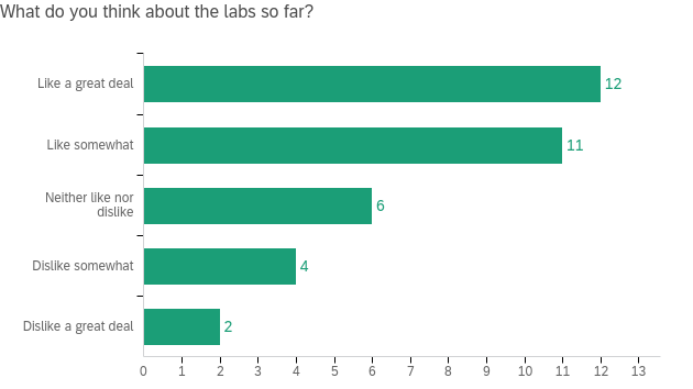
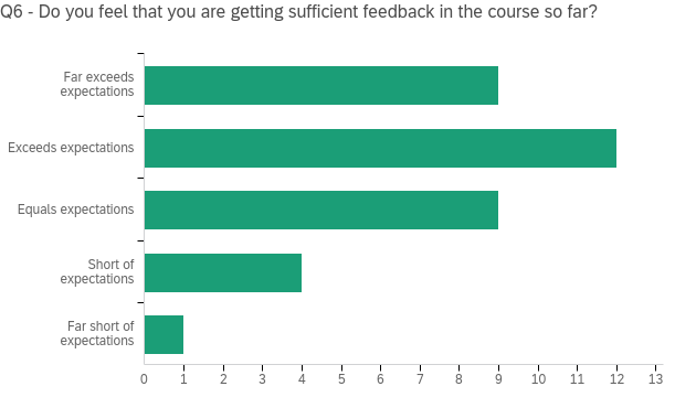
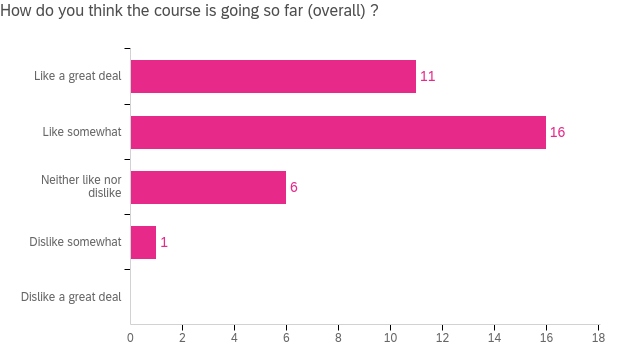
Feedback Results
Lab 2 Optional Question
Miscellaneous stuff for Lab 3
- Generating Random numbers
- Exploring numpy documentation
Aggregation and Grouping

Feedback Results¶

Lab 2 Optional Question¶

3.3: Create a Python program that takes a string text and calculates the frequency of each character (6 marks)¶

text = “””Elephants are mammals of the family Elephantidae and the largest existing land animals. Three species are currently recognised: the African bush elephant, the African forest elephant, and the Asian elephant. Elephantidae is the only surviving family of the order Proboscidea; extinct members include the mastodons. The family Elephantidae also contains several now-extinct groups, including the mammoths and straight-tusked elephants. African elephants have larger ears and concave backs, whereas Asian elephants have smaller ears, and convex or level backs. Distinctive features of all elephants include a long trunk, tusks, large ear flaps, massive legs, and tough but sensitive skin. The trunk, also called a proboscis, is used for breathing, bringing food and water to the mouth, and grasping objects. Tusks, which are derived from the incisor teeth, serve both as weapons and as tools for moving objects and digging. The large ear flaps assist in maintaining a constant body temperature as well as in communication. The pillar-like legs carry their great weight. Elephants are scattered throughout sub-Saharan Africa, South Asia, and Southeast Asia and are found in different habitats, including savannahs, forests, deserts, and marshes. They are herbivorous, and they stay near water when it is accessible. They are considered to be keystone species, due to their impact on their environments.[1] Other animals tend to keep their distance from elephants; the exception is their predators such as lions, tigers, hyenas, and wild dogs, which usually target only young elephants (calves). Elephants have a fission–fusion society, in which multiple family groups come together to socialise. Females (cows) tend to live in family groups, which can consist of one female with her calves or several related females with offspring. The groups, which do not include bulls, are led by the (usually) oldest cow, known as the matriarch.”””

Hint: There are many ways to do this, the most “elegant” way uses a mixture of sets, and the Counter modules from collections

Sample output:¶

‘ ‘: Count of 293 and Percentage of 15.2%
‘(‘: Count of 3 and Percentage of 0.2%
‘)’: Count of 3 and Percentage of 0.2%
‘,’: Count of 32 and Percentage of 1.7%
‘-‘: Count of 4 and Percentage of 0.2%
‘.’: Count of 17 and Percentage of 0.9%
‘1’: Count of 1 and Percentage of 0.1%
‘:’: Count of 1 and Percentage of 0.1%
‘;’: Count of 2 and Percentage of 0.1%
‘A’: Count of 8 and Percentage of 0.4%
‘D’: Count of 1 and Percentage of 0.1%
‘E’: Count of 6 and Percentage of 0.3%
‘F’: Count of 1 and Percentage of 0.1%
‘O’: Count of 1 and Percentage of 0.1%
‘P’: Count of 1 and Percentage of 0.1%
‘S’: Count of 3 and Percentage of 0.2%
‘T’: Count of 9 and Percentage of 0.5%
‘[‘: Count of 1 and Percentage of 0.1%
‘]’: Count of 1 and Percentage of 0.1%
‘a’: Count of 147 and Percentage of 7.6%
‘b’: Count of 20 and Percentage of 1.0%
‘c’: Count of 55 and Percentage of 2.8%
‘d’: Count of 53 and Percentage of 2.7%
‘e’: Count of 189 and Percentage of 9.8%
‘f’: Count of 32 and Percentage of 1.7%
‘g’: Count of 37 and Percentage of 1.9%
‘h’: Count of 84 and Percentage of 4.4%
‘i’: Count of 109 and Percentage of 5.6%
‘j’: Count of 2 and Percentage of 0.1%
‘k’: Count of 12 and Percentage of 0.6%
‘l’: Count of 80 and Percentage of 4.1%
‘m’: Count of 35 and Percentage of 1.8%
‘n’: Count of 114 and Percentage of 5.9%
‘o’: Count of 87 and Percentage of 4.5%
‘p’: Count of 34 and Percentage of 1.8%
‘r’: Count of 92 and Percentage of 4.8%
‘s’: Count of 131 and Percentage of 6.8%
‘t’: Count of 120 and Percentage of 6.2%
‘u’: Count of 41 and Percentage of 2.1%
‘v’: Count of 22 and Percentage of 1.1%
‘w’: Count of 19 and Percentage of 1.0%
‘x’: Count of 5 and Percentage of 0.3%
‘y’: Count of 21 and Percentage of 1.1%
‘–’: Count of 1 and Percentage of 0.1%

Hint: There are many ways to do this, the most “elegant” way uses a mixture of sets, and the Counter modules from collections

text = """Elephants are mammals of the family Elephantidae and the largest existing land animals. Three species are currently recognised: the African bush elephant, the African forest elephant, and the Asian elephant. Elephantidae is the only surviving family of the order Proboscidea; extinct members include the mastodons. The family Elephantidae also contains several now-extinct groups, including the mammoths and straight-tusked elephants. African elephants have larger ears and concave backs, whereas Asian elephants have smaller ears, and convex or level backs. Distinctive features of all elephants include a long trunk, tusks, large ear flaps, massive legs, and tough but sensitive skin. The trunk, also called a proboscis, is used for breathing, bringing food and water to the mouth, and grasping objects. Tusks, which are derived from the incisor teeth, serve both as weapons and as tools for moving objects and digging. The large ear flaps assist in maintaining a constant body temperature as well as in communication. The pillar-like legs carry their great weight. Elephants are scattered throughout sub-Saharan Africa, South Asia, and Southeast Asia and are found in different habitats, including savannahs, forests, deserts, and marshes. They are herbivorous, and they stay near water when it is accessible. They are considered to be keystone species, due to their impact on their environments.[1] Other animals tend to keep their distance from elephants; the exception is their predators such as lions, tigers, hyenas, and wild dogs, which usually target only young elephants (calves). Elephants have a fission–fusion society, in which multiple family groups come together to socialise. Females (cows) tend to live in family groups, which can consist of one female with her calves or several related females with offspring. The groups, which do not include bulls, are led by the (usually) oldest cow, known as the matriarch."""

letters = list(set(text.lower())) # I think it makes more sense to combine the capital and the lower-case letters

len(letters)

text_length = len(text)
for l in sorted(letters):
    lcount = text.lower().count(l)
    print(f"For the character '{l}': Count of {lcount} and Percentage of {100*lcount/text_length:.1f} %")
    
# this solution was inspired by this SO post: https://stackoverflow.com/a/1155648

For the character ' ': Count of 293 and Percentage of 15.2 %
For the character '(': Count of 3 and Percentage of 0.2 %
For the character ')': Count of 3 and Percentage of 0.2 %
For the character ',': Count of 32 and Percentage of 1.7 %
For the character '-': Count of 4 and Percentage of 0.2 %
For the character '.': Count of 17 and Percentage of 0.9 %
For the character '1': Count of 1 and Percentage of 0.1 %
For the character ':': Count of 1 and Percentage of 0.1 %
For the character ';': Count of 2 and Percentage of 0.1 %
For the character '[': Count of 1 and Percentage of 0.1 %
For the character ']': Count of 1 and Percentage of 0.1 %
For the character 'a': Count of 155 and Percentage of 8.0 %
For the character 'b': Count of 20 and Percentage of 1.0 %
For the character 'c': Count of 55 and Percentage of 2.8 %
For the character 'd': Count of 54 and Percentage of 2.8 %
For the character 'e': Count of 195 and Percentage of 10.1 %
For the character 'f': Count of 33 and Percentage of 1.7 %
For the character 'g': Count of 37 and Percentage of 1.9 %
For the character 'h': Count of 84 and Percentage of 4.4 %
For the character 'i': Count of 109 and Percentage of 5.6 %
For the character 'j': Count of 2 and Percentage of 0.1 %
For the character 'k': Count of 12 and Percentage of 0.6 %
For the character 'l': Count of 80 and Percentage of 4.1 %
For the character 'm': Count of 35 and Percentage of 1.8 %
For the character 'n': Count of 114 and Percentage of 5.9 %
For the character 'o': Count of 88 and Percentage of 4.6 %
For the character 'p': Count of 35 and Percentage of 1.8 %
For the character 'r': Count of 92 and Percentage of 4.8 %
For the character 's': Count of 134 and Percentage of 6.9 %
For the character 't': Count of 129 and Percentage of 6.7 %
For the character 'u': Count of 41 and Percentage of 2.1 %
For the character 'v': Count of 22 and Percentage of 1.1 %
For the character 'w': Count of 19 and Percentage of 1.0 %
For the character 'x': Count of 5 and Percentage of 0.3 %
For the character 'y': Count of 21 and Percentage of 1.1 %
For the character '–': Count of 1 and Percentage of 0.1 %

Miscellaneous stuff from Lab 3¶

Generating Random numbers
Exploring numpy documentation

import random
import numpy as np

# for loop method
rints= []
for i in range(10):
    rints.append(random.randrange(5,50))

# list comprehension method

[random.randrange(5,50) for i in range(10)]

[11, 27, 25, 14, 11, 40, 14, 24, 17, 44]

# another way
np.random.rand(10)

array([0.09606352, 0.45121143, 0.87241139, 0.47308334, 0.09519842,
       0.73981544, 0.09593441, 0.36333275, 0.32305733, 0.48241197])

# another way
rints2 = np.arange(5,50)

for i in range(10):
    print(random.choice(rints2))

random.choice(rints)

Aggregation and Grouping¶

Attribution¶

This notebook contains an excerpt from the Python Data Science Handbook by Jake VanderPlas; the content is available on GitHub.

The text is released under the CC-BY-NC-ND license, and code is released under the MIT license. If you find this content useful, please consider supporting the work by buying the book!

An essential piece of analysis of large data is efficient summarization: computing aggregations like sum(), mean(), median(), min(), and max(), in which a single number gives insight into the nature of a potentially large dataset. In this section, we’ll explore aggregations in Pandas, from simple operations akin to what we’ve seen on NumPy arrays, to more sophisticated operations based on the concept of a groupby.

For convenience, we’ll use the same display magic function that we’ve seen in previous sections:

import numpy as np
import pandas as pd

class display(object):
    """Display HTML representation of multiple objects"""
    template = """<div style="float: left; padding: 10px;">
    <p style='font-family:"Courier New", Courier, monospace'>{0}</p>{1}
    </div>"""
    def __init__(self, *args):
        self.args = args
        
    def _repr_html_(self):
        return '\n'.join(self.template.format(a, eval(a)._repr_html_())
                         for a in self.args)
    
    def __repr__(self):
        return '\n\n'.join(a + '\n' + repr(eval(a))
                           for a in self.args)

Planets Data¶

Here we will use the Planets dataset, available via the Seaborn package (see Visualization With Seaborn). It gives information on planets that astronomers have discovered around other stars (known as extrasolar planets or exoplanets for short). It can be downloaded with a simple Seaborn command:

import seaborn as sns # `conda install seaborn` in your terminal
planets = sns.load_dataset('planets')
planets

	method	number	orbital_period	mass	distance	year
0	Radial Velocity	1	269.300000	7.10	77.40	2006
1	Radial Velocity	1	874.774000	2.21	56.95	2008
2	Radial Velocity	1	763.000000	2.60	19.84	2011
3	Radial Velocity	1	326.030000	19.40	110.62	2007
4	Radial Velocity	1	516.220000	10.50	119.47	2009
...	...	...	...	...	...	...
1030	Transit	1	3.941507	NaN	172.00	2006
1031	Transit	1	2.615864	NaN	148.00	2007
1032	Transit	1	3.191524	NaN	174.00	2007
1033	Transit	1	4.125083	NaN	293.00	2008
1034	Transit	1	4.187757	NaN	260.00	2008

1035 rows × 6 columns

planets.head()

	method	number	orbital_period	mass	distance	year
0	Radial Velocity	1	269.300	7.10	77.40	2006
1	Radial Velocity	1	874.774	2.21	56.95	2008
2	Radial Velocity	1	763.000	2.60	19.84	2011
3	Radial Velocity	1	326.030	19.40	110.62	2007
4	Radial Velocity	1	516.220	10.50	119.47	2009

This has some details on the 1,000+ extrasolar planets discovered up to 2014.

Simple Aggregation in Pandas¶

Earlier, we explored some of the data aggregations available for NumPy arrays (“Aggregations: Min, Max, and Everything In Between”). As with a one-dimensional NumPy array, for a Pandas Series the aggregates return a single value:

rng = np.random.RandomState(42)
ser = pd.Series(rng.rand(5))
ser

  0.374540
  0.950714
  0.731994
  0.598658
  0.156019
dtype: float64

ser.sum()

2.811925491708157

ser.mean()

0.5623850983416314

For a DataFrame, by default the aggregates return results within each column:

import pandas as pd

df = pd.DataFrame({'A': rng.rand(5),
                   'B': rng.rand(5)})
df

	A	B
0	0.155995	0.020584
1	0.058084	0.969910
2	0.866176	0.832443
3	0.601115	0.212339
4	0.708073	0.181825

df.mean()

A    0.477888
B    0.443420
dtype: float64

By specifying the axis argument, you can instead aggregate within each row:

df.mean(axis='columns')

  0.088290
  0.513997
  0.849309
  0.406727
  0.444949
dtype: float64

Pandas Series and DataFrames include all of the common aggregates mentioned in Aggregations: Min, Max, and Everything In Between; in addition, there is a convenience method describe() that computes several common aggregates for each column and returns the result. Let’s use this on the Planets data, for now dropping rows with missing values:

planets.dropna().describe()

	number	orbital_period	mass	distance	year
count	498.00000	498.000000	498.000000	498.000000	498.000000
mean	1.73494	835.778671	2.509320	52.068213	2007.377510
std	1.17572	1469.128259	3.636274	46.596041	4.167284
min	1.00000	1.328300	0.003600	1.350000	1989.000000
25%	1.00000	38.272250	0.212500	24.497500	2005.000000
50%	1.00000	357.000000	1.245000	39.940000	2009.000000
75%	2.00000	999.600000	2.867500	59.332500	2011.000000
max	6.00000	17337.500000	25.000000	354.000000	2014.000000

This can be a useful way to begin understanding the overall properties of a dataset. For example, we see in the year column that although exoplanets were discovered as far back as 1989, half of all known expolanets were not discovered until 2010 or after. This is largely thanks to the Kepler mission, which is a space-based telescope specifically designed for finding eclipsing planets around other stars.

The following table summarizes some other built-in Pandas aggregations:

Aggregation	Description
`count()`	Total number of items
`first()`, `last()`	First and last item
`mean()`, `median()`	Mean and median
`min()`, `max()`	Minimum and maximum
`std()`, `var()`	Standard deviation and variance
`mad()`	Mean absolute deviation
`prod()`	Product of all items
`sum()`	Sum of all items

These are all methods of DataFrame and Series objects.

To go deeper into the data, however, simple aggregates are often not enough. The next level of data summarization is the groupby operation, which allows you to quickly and efficiently compute aggregates on subsets of data.

Break - back at 1 PM!¶

GroupBy: Split, Apply, Combine¶

Simple aggregations can give you a flavor of your dataset, but often we would prefer to aggregate conditionally on some label or index: this is implemented in the so-called groupby operation. The name “group by” comes from a command in the SQL database language, but it is perhaps more illuminative to think of it in the terms first coined by Hadley Wickham of Rstats fame: split, apply, combine.

Split, apply, combine¶

A canonical example of this split-apply-combine operation, where the “apply” is a summation aggregation, is illustrated in this figure:

figure source in Appendix

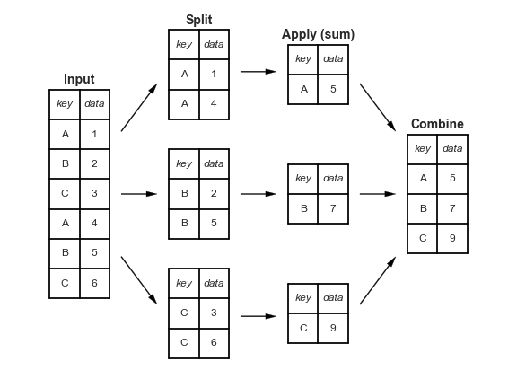
This makes clear what the groupby accomplishes:

The split step involves breaking up and grouping a DataFrame depending on the value of the specified key.
The apply step involves computing some function, usually an aggregate, transformation, or filtering, within the individual groups.
The combine step merges the results of these operations into an output array.

While this could certainly be done manually using some combination of the masking, aggregation, and merging commands covered earlier, an important realization is that the intermediate splits do not need to be explicitly instantiated. Rather, the GroupBy can (often) do this in a single pass over the data, updating the sum, mean, count, min, or other aggregate for each group along the way. The power of the GroupBy is that it abstracts away these steps: the user need not think about how the computation is done under the hood, but rather thinks about the operation as a whole.

As a concrete example, let’s take a look at using Pandas for the computation shown in this diagram. We’ll start by creating the input DataFrame:

df = pd.DataFrame({'key': ['A', 'B', 'C', 'A', 'B', 'C'],
                   'data': range(6)}, columns=['key', 'data'])
df

	key	data
0	A	0
1	B	1
2	C	2
3	A	3
4	B	4
5	C	5

The most basic split-apply-combine operation can be computed with the groupby() method of DataFrames, passing the name of the desired key column:

df.groupby('key')

<pandas.core.groupby.generic.DataFrameGroupBy object at 0x7fdab1254190>

Notice that what is returned is not a set of DataFrames, but a DataFrameGroupBy object. This object is where the magic is: you can think of it as a special view of the DataFrame, which is poised to dig into the groups but does no actual computation until the aggregation is applied. This “lazy evaluation” approach means that common aggregates can be implemented very efficiently in a way that is almost transparent to the user.

To produce a result, we can apply an aggregate to this DataFrameGroupBy object, which will perform the appropriate apply/combine steps to produce the desired result:

df.groupby('key').sum()

	data
key
A	3
B	5
C	7

The sum() method is just one possibility here; you can apply virtually any common Pandas or NumPy aggregation function, as well as virtually any valid DataFrame operation, as we will see in the following discussion.

The GroupBy object¶

The GroupBy object is a very flexible abstraction. In many ways, you can simply treat it as if it’s a collection of DataFrames, and it does the difficult things under the hood. Let’s see some examples using the Planets data.

Perhaps the most important operations made available by a GroupBy are aggregate, filter, transform, and apply. We’ll discuss each of these more fully in “Aggregate, Filter, Transform, Apply”, but before that let’s introduce some of the other functionality that can be used with the basic GroupBy operation.

Column indexing¶

The GroupBy object supports column indexing in the same way as the DataFrame, and returns a modified GroupBy object. For example:

planets

	method	number	orbital_period	mass	distance	year
0	Radial Velocity	1	269.300000	7.10	77.40	2006
1	Radial Velocity	1	874.774000	2.21	56.95	2008
2	Radial Velocity	1	763.000000	2.60	19.84	2011
3	Radial Velocity	1	326.030000	19.40	110.62	2007
4	Radial Velocity	1	516.220000	10.50	119.47	2009
...	...	...	...	...	...	...
1030	Transit	1	3.941507	NaN	172.00	2006
1031	Transit	1	2.615864	NaN	148.00	2007
1032	Transit	1	3.191524	NaN	174.00	2007
1033	Transit	1	4.125083	NaN	293.00	2008
1034	Transit	1	4.187757	NaN	260.00	2008

1035 rows × 6 columns

planets.groupby('method') 

<pandas.core.groupby.generic.DataFrameGroupBy object at 0x7fdab12542e0>

planets.groupby('method')['orbital_period']

<pandas.core.groupby.generic.SeriesGroupBy object at 0x7fdaf4f8f8e0>

Here we’ve selected a particular Series group from the original DataFrame group by reference to its column name. As with the GroupBy object, no computation is done until we call some aggregate on the object:

planets.groupby('method')['orbital_period'].median()

method
Astrometry                         631.180000
Eclipse Timing Variations         4343.500000
Imaging                          27500.000000
Microlensing                      3300.000000
Orbital Brightness Modulation        0.342887
Pulsar Timing                       66.541900
Pulsation Timing Variations       1170.000000
Radial Velocity                    360.200000
Transit                              5.714932
Transit Timing Variations           57.011000
Name: orbital_period, dtype: float64

This gives an idea of the general scale of orbital periods (in days) that each method is sensitive to.

Iteration over groups¶

The GroupBy object supports direct iteration over the groups, returning each group as a Series or DataFrame:

for (method, group) in planets.groupby('method'):
    print(f"{method:30s} shape={group.shape}")

Astrometry                     shape=(2, 6)
Eclipse Timing Variations      shape=(9, 6)
Imaging                        shape=(38, 6)
Microlensing                   shape=(23, 6)
Orbital Brightness Modulation  shape=(3, 6)
Pulsar Timing                  shape=(5, 6)
Pulsation Timing Variations    shape=(1, 6)
Radial Velocity                shape=(553, 6)
Transit                        shape=(397, 6)
Transit Timing Variations      shape=(4, 6)

This can be useful for doing certain things manually, though it is often much faster to use the built-in apply functionality, which we will discuss momentarily.

Dispatch methods¶

Through some Python class magic, any method not explicitly implemented by the GroupBy object will be passed through and called on the groups, whether they are DataFrame or Series objects. For example, you can use the describe() method of DataFrames to perform a set of aggregations that describe each group in the data:

planets.groupby('method')['year'].describe().unstack()

       method                       
count  Astrometry                          2.0
       Eclipse Timing Variations           9.0
       Imaging                            38.0
       Microlensing                       23.0
       Orbital Brightness Modulation       3.0
                                         ...  
max    Pulsar Timing                    2011.0
       Pulsation Timing Variations      2007.0
       Radial Velocity                  2014.0
       Transit                          2014.0
       Transit Timing Variations        2014.0
Length: 80, dtype: float64

Looking at this table helps us to better understand the data: for example, the vast majority of planets have been discovered by the Radial Velocity and Transit methods, though the latter only became common (due to new, more accurate telescopes) in the last decade. The newest methods seem to be Transit Timing Variation and Orbital Brightness Modulation, which were not used to discover a new planet until 2011.

This is just one example of the utility of dispatch methods. Notice that they are applied to each individual group, and the results are then combined within GroupBy and returned. Again, any valid DataFrame/Series method can be used on the corresponding GroupBy object, which allows for some very flexible and powerful operations!

Aggregate, filter, transform, apply¶

The preceding discussion focused on aggregation for the combine operation, but there are more options available. In particular, GroupBy objects have aggregate(), filter(), transform(), and apply() methods that efficiently implement a variety of useful operations before combining the grouped data.

For the purpose of the following subsections, we’ll use this DataFrame:

rng = np.random.RandomState(0)
df = pd.DataFrame({'key': ['A', 'B', 'C', 'A', 'B', 'C'],
                   'data1': range(6),
                   'data2': rng.randint(0, 10, 6)},
                   columns = ['key', 'data1', 'data2'])
df

	key	data1	data2
0	A	0	5
1	B	1	0
2	C	2	3
3	A	3	3
4	B	4	7
5	C	5	9

Aggregation¶

We’re now familiar with GroupBy aggregations with sum(), median(), and the like, but the aggregate() method allows for even more flexibility. It can take a string, a function, or a list thereof, and compute all the aggregates at once. Here is a quick example combining all these:

df.groupby('key').aggregate(['min', np.median, max])

	data1			data2
	min	median	max	min	median	max
key
A	0	1.5	3	3	4.0	5
B	1	2.5	4	0	3.5	7
C	2	3.5	5	3	6.0	9

Another useful pattern is to pass a dictionary mapping column names to operations to be applied on that column:

df.groupby('key').aggregate({'data1': 'min',
                             'data2': 'max'})

	data1	data2
key
A	0	5
B	1	7
C	2	9

Filtering¶

A filtering operation allows you to drop data based on the group properties. For example, we might want to keep all groups in which the standard deviation is larger than some critical value:

def filter_func(x):
    return x['data2'].std() > 4

display('df', "df.groupby('key').std()", "df.groupby('key').filter(filter_func)")

df

	key	data1	data2
0	A	0	5
1	B	1	0
2	C	2	3
3	A	3	3
4	B	4	7
5	C	5	9

df.groupby('key').std()

	data1	data2
key
A	2.12132	1.414214
B	2.12132	4.949747
C	2.12132	4.242641

df.groupby('key').filter(filter_func)

	key	data1	data2
1	B	1	0
2	C	2	3
4	B	4	7
5	C	5	9

The filter function should return a Boolean value specifying whether the group passes the filtering. Here because group A does not have a standard deviation greater than 4, it is dropped from the result.

Transformation¶

While aggregation must return a reduced version of the data, transformation can return some transformed version of the full data to recombine. For such a transformation, the output is the same shape as the input. A common example is to center the data by subtracting the group-wise mean:

df.groupby('key').transform(lambda x: x - x.mean())

	data1	data2
0	-1.5	1.0
1	-1.5	-3.5
2	-1.5	-3.0
3	1.5	-1.0
4	1.5	3.5
5	1.5	3.0

The apply() method¶

The apply() method lets you apply an arbitrary function to the group results. The function should take a DataFrame, and return either a Pandas object (e.g., DataFrame, Series) or a scalar; the combine operation will be tailored to the type of output returned.

For example, here is an apply() that normalizes the first column by the sum of the second:

def norm_by_data2(x):
    # x is a DataFrame of group values
    x['data1'] /= x['data2'].sum() # "y/= something" is equivalent to "y = y/something"
    return x

display('df', "df.groupby('key').apply(norm_by_data2)")

df

	key	data1	data2
0	A	0	5
1	B	1	0
2	C	2	3
3	A	3	3
4	B	4	7
5	C	5	9

df.groupby('key').apply(norm_by_data2)

	key	data1	data2
0	A	0.000000	5
1	B	0.142857	0
2	C	0.166667	3
3	A	0.375000	3
4	B	0.571429	7
5	C	0.416667	9

apply() within a GroupBy is quite flexible: the only criterion is that the function takes a DataFrame and returns a Pandas object or scalar; what you do in the middle is up to you!

Specifying the split key¶

In the simple examples presented before, we split the DataFrame on a single column name. This is just one of many options by which the groups can be defined, and we’ll go through some other options for group specification here.

A list, array, series, or index providing the grouping keys¶

The key can be any series or list with a length matching that of the DataFrame. For example:

L = [0, 1, 0, 1, 2, 0]
display('df', 'df.groupby(L).sum()')

df

	key	data1	data2
0	A	0	5
1	B	1	0
2	C	2	3
3	A	3	3
4	B	4	7
5	C	5	9

df.groupby(L).sum()

	data1	data2
0	7	17
1	4	3
2	4	7

Of course, this means there’s another, more verbose way of accomplishing the df.groupby('key') from before:

display('df', "df.groupby(df['key']).sum()")

df

	key	data1	data2
0	A	0	5
1	B	1	0
2	C	2	3
3	A	3	3
4	B	4	7
5	C	5	9

df.groupby(df['key']).sum()

	data1	data2
key
A	3	8
B	5	7
C	7	12

A dictionary or series mapping index to group¶

Another method is to provide a dictionary that maps index values to the group keys:

df2 = df.set_index('key')
mapping = {'A': 'vowel', 'B': 'consonant', 'C': 'consonant'}
display('df2', 'df2.groupby(mapping).sum()')

df2

	data1	data2
key
A	0	5
B	1	0
C	2	3
A	3	3
B	4	7
C	5	9

df2.groupby(mapping).sum()

	data1	data2
key
consonant	12	19
vowel	3	8

Any Python function¶

Similar to mapping, you can pass any Python function that will input the index value and output the group:

display('df2', 'df2.groupby(str.lower).mean()')

df2

	data1	data2
key
A	0	5
B	1	0
C	2	3
A	3	3
B	4	7
C	5	9

df2.groupby(str.lower).mean()

	data1	data2
key
a	1.5	4.0
b	2.5	3.5
c	3.5	6.0

A list of valid keys¶

Further, any of the preceding key choices can be combined to group on a multi-index:

df2.groupby([str.lower, mapping]).mean()

		data1	data2
key	key
a	vowel	1.5	4.0
b	consonant	2.5	3.5
c	consonant	3.5	6.0

Grouping example¶

As an example of this, in a couple lines of Python code we can put all these together and count discovered planets by method and by decade:

planets

	method	number	orbital_period	mass	distance	year
0	Radial Velocity	1	269.300000	7.10	77.40	2006
1	Radial Velocity	1	874.774000	2.21	56.95	2008
2	Radial Velocity	1	763.000000	2.60	19.84	2011
3	Radial Velocity	1	326.030000	19.40	110.62	2007
4	Radial Velocity	1	516.220000	10.50	119.47	2009
...	...	...	...	...	...	...
1030	Transit	1	3.941507	NaN	172.00	2006
1031	Transit	1	2.615864	NaN	148.00	2007
1032	Transit	1	3.191524	NaN	174.00	2007
1033	Transit	1	4.125083	NaN	293.00	2008
1034	Transit	1	4.187757	NaN	260.00	2008

1035 rows × 6 columns

decade = 10 * (planets['year'] // 10)
decade

     2000
     2000
     2010
     2000
     2000
        ... 
  2000
  2000
  2000
  2000
  2000
Name: year, Length: 1035, dtype: int64

decade = decade.astype(str) + 's'
decade

     2000s
     2000s
     2010s
     2000s
     2000s
        ...  
  2000s
  2000s
  2000s
  2000s
  2000s
Name: year, Length: 1035, dtype: object

decade.name = 'decade'

planets.groupby(['method', decade])['number'].sum().unstack().fillna(0)

decade	1980s	1990s	2000s	2010s
method
Astrometry	0.0	0.0	0.0	2.0
Eclipse Timing Variations	0.0	0.0	5.0	10.0
Imaging	0.0	0.0	29.0	21.0
Microlensing	0.0	0.0	12.0	15.0
Orbital Brightness Modulation	0.0	0.0	0.0	5.0
Pulsar Timing	0.0	9.0	1.0	1.0
Pulsation Timing Variations	0.0	0.0	1.0	0.0
Radial Velocity	1.0	52.0	475.0	424.0
Transit	0.0	0.0	64.0	712.0
Transit Timing Variations	0.0	0.0	0.0	9.0

This shows the power of combining many of the operations we’ve discussed up to this point when looking at realistic datasets. We immediately gain a coarse understanding of when and how planets have been discovered over the past several decades!

Here I would suggest digging into these few lines of code, and evaluating the individual steps to make sure you understand exactly what they are doing to the result. It’s certainly a somewhat complicated example, but understanding these pieces will give you the means to similarly explore your own data.

That’s it!

Have a good weekend!

DATA 301

Class 3C - Data Wrangling with Pandas III¶

Class Outline¶

Feedback Results¶

Lab 2 Optional Question¶

3.3: Create a Python program that takes a string text and calculates the frequency of each character (6 marks)¶

Sample output:¶

Miscellaneous stuff from Lab 3¶

Aggregation and Grouping¶

Attribution¶

Planets Data¶

Simple Aggregation in Pandas¶

Break - back at 1 PM!¶

GroupBy: Split, Apply, Combine¶

Split, apply, combine¶

The GroupBy object¶

Column indexing¶

Iteration over groups¶

Dispatch methods¶

Aggregate, filter, transform, apply¶

Aggregation¶

Filtering¶

Transformation¶

The apply() method¶

Specifying the split key¶

A list, array, series, or index providing the grouping keys¶

A dictionary or series mapping index to group¶

Any Python function¶

A list of valid keys¶

Grouping example¶