Introduction to Altair#

# Import libraries

import pandas as pd
import numpy as np
from IPython.display import IFrame

import matplotlib.pyplot as plt

import altair as alt
from vega_datasets import data
mtcars = data.cars()

# Poll question links
q1 = 'https://app.sli.do/event/0nwvmaj5/embed/polls/5cff1bff-b850-4647-b2fd-c799dbd16b78'
q2 = 'https://app.sli.do/event/0nwvmaj5/embed/polls/e3282762-367b-40c7-a9cc-c76f9f8db849'

## Set Altair default size

def theme_fm(*args, **kwargs):
    return {'height': 220,
            'width' : 220,
            'config': {'style': {'circle': {'size': 400},
                                'point': {'size': 30},
                                'square': {'size': 400},
                                },
                       'legend': {'symbolSize': 20, 'titleFontSize': 20, 'labelFontSize': 20}, 
                       'axis': {'titleFontSize': 20, 'labelFontSize': 20}},
            }

alt.themes.register('theme_fm', theme_fm)
alt.themes.enable('theme_fm')

print('You are ready to proceed!')

You are ready to proceed!

Learning Context#

Altair: Declarative Visualization in Python#

Firas Moosvi

## We'll be using the mtcars dataset for most of the cool stuff in this lecture
mtcars.head()

	Name	Miles_per_Gallon	Cylinders	Displacement	Horsepower	Weight_in_lbs	Acceleration	Year	Origin
0	chevrolet chevelle malibu	18.0	8	307.0	130.0	3504	12.0	1970-01-01	USA
1	buick skylark 320	15.0	8	350.0	165.0	3693	11.5	1970-01-01	USA
2	plymouth satellite	18.0	8	318.0	150.0	3436	11.0	1970-01-01	USA
3	amc rebel sst	16.0	8	304.0	150.0	3433	12.0	1970-01-01	USA
4	ford torino	17.0	8	302.0	140.0	3449	10.5	1970-01-01	USA

Learning Objectives#

Explain the difference between declarative and imperative syntax

Describe the 6 components of the visualization grammar

Construct data visualizations using Altair

Add interactivity to Altair plots

Start critically evaluate data visualizations

Starting with the punchline!#

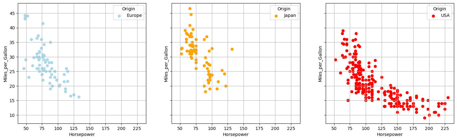
By the end of lecture today, you will learn how to make this chart using the mtcars dataset:

base = alt.Chart(mtcars).mark_point().encode(
    alt.X('Horsepower'),
    alt.Y('Miles_per_Gallon'),
    alt.Color('Origin'),
    alt.Column('Origin')
) 

base.interactive()

In matplotlib:#

If you’re familiar with matplotlib, this should illustrate to you how Altair is different - not better or worse, just differently sane (h/t Greg Wilson).

colour_map = dict(zip(mtcars['Origin'].unique(), ['red','lightblue','orange']))
n_panels = len(colour_map)

fig, ax = plt.subplots(1, n_panels, figsize=(n_panels * 6, 5),
                       sharex = True, sharey = True)

for i, (country,group) in enumerate(mtcars.groupby('Origin')):
    ax[i].scatter(group['Horsepower'],
                  group['Miles_per_Gallon'],
                  label = country,
                  color = colour_map[country])
    ax[i].legend(title='Origin')
    ax[i].grid()
    ax[i].set_xlabel('Horsepower')
    ax[i].set_ylabel('Miles_per_Gallon')

Part 1: Introduction to Altair#

Slide used with permission from Eitan Lees

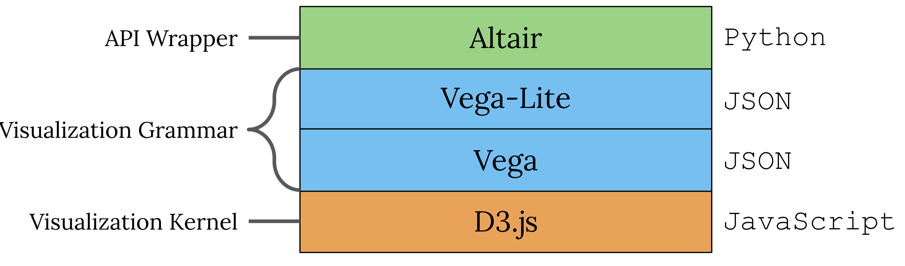
Why do we need a visualization grammar?#

# Altair: Declarative

base = alt.Chart(mtcars).mark_point().encode(
    alt.X('Horsepower'),
    alt.Y('Miles_per_Gallon'),
    alt.Color('Origin'),
    alt.Column('Origin')
)

base

# Matplotlib: Imperative

colour_map = dict(zip(mtcars['Origin'].unique(), ['red','lightblue','orange']))
n_panels = len(colour_map)

fig, ax = plt.subplots(1, n_panels, figsize=(n_panels * 6, 5),
                       sharex = True, sharey = True)

for i, (country,group) in enumerate(mtcars.groupby('Origin')):
    ax[i].scatter(group['Horsepower'],
                  group['Miles_per_Gallon'],
                  label = country,
                  color = colour_map[country])
    ax[i].legend(title='Origin')
    ax[i].grid()
    ax[i].set_xlabel('Horsepower')
    ax[i].set_ylabel('Miles_per_Gallon')

Slide used with permission from Eitan Lees

1. Tabular Data#

Data in Altair is built around the Pandas DataFrame.

The fundamental object in Altair is the Chart. It takes the dataframe as a single argument:

chart = alt.Chart(DataFrame)

Let’s create a simple DataFrame to visualize, with a categorical data in the Letters column and numerical data in the Numbers column:

df = pd.DataFrame({'Letters': list('CCCDDDEEE'),
                     'Numbers': [2, 7, 4, 1, 2, 6, 8, 4, 7]})
df

	Letters	Numbers
0	C	2
1	C	7
2	C	4
3	D	1
4	D	2
5	D	6
6	E	8
7	E	4
8	E	7

plot = alt.Chart(df)

plot 

---------------------------------------------------------------------------
SchemaValidationError                     Traceback (most recent call last)
File /opt/hostedtoolcache/Python/3.9.13/x64/lib/python3.9/site-packages/altair/vegalite/v4/api.py:2020, in Chart.to_dict(self, *args, **kwargs)
   2018     copy.data = core.InlineData(values=[{}])
   2019     return super(Chart, copy).to_dict(*args, **kwargs)
-> 2020 return super().to_dict(*args, **kwargs)

File /opt/hostedtoolcache/Python/3.9.13/x64/lib/python3.9/site-packages/altair/vegalite/v4/api.py:393, in TopLevelMixin.to_dict(self, *args, **kwargs)
    391 if dct is None:
    392     kwargs["validate"] = "deep"
--> 393     dct = super(TopLevelMixin, copy).to_dict(*args, **kwargs)
    395 # TODO: following entries are added after validation. Should they be validated?
    396 if is_top_level:
    397     # since this is top-level we add $schema if it's missing

File /opt/hostedtoolcache/Python/3.9.13/x64/lib/python3.9/site-packages/altair/utils/schemapi.py:340, in SchemaBase.to_dict(self, validate, ignore, context)
    338         self.validate(result)
    339     except jsonschema.ValidationError as err:
--> 340         raise SchemaValidationError(self, err)
    341 return result

SchemaValidationError: Invalid specification

        altair.vegalite.v4.api.Chart, validating 'required'

        'mark' is a required property
        

alt.Chart(...)

Slide used with permission from Eitan Lees

2. Chart Marks#

Next we can decide what sort of mark we would like to use to represent our data.

Here are some of the more commonly used mark_*() methods supported in Altair and Vega-Lite; for more detail see Marks in the Altair documentation:

Mark
`mark_area()`
`mark_bar()`
`mark_circle()`, `mark_point`, `mark_square`
`mark_rect()`
`mark_line()`
`mark_rule()`
`mark_text()`
`mark_image()`

Let’s add a mark_point() to our plot:

plot = alt.Chart(df).mark_point()

plot

😒

We have a plot now, but clearly we’re being pranked: all the data points collapsed to one location! Why ?

Slide used with permission from Eitan Lees

A visual encoding specifies how a given data column should be mapped onto visual properties of the visualization.

Some of the more frequently used visual encodings are listed on the right:

For a complete list of these encodings, see the Encodings section of the documentation.

Encoding	What does it encode?
`X`	x-axis value
`Y`	y-axis value
`Color`	color of the mark
`Opacity`	transparency/opacity of the mark
`Shape`	shape of the mark
`Size`	size of the mark
`Row`	row within a grid of facet plots
`Column`	column within a grid of facet plots

Let’s add an encoding so the data is mapped to the x and y axes:

plot = alt.Chart(df).mark_point().encode(alt.X('Numbers'))

plot

# We still haven't encoded any of the data to the Y-axis!

You Try!#

Encode the Letters column at the y position to make the visualization more useful.

plot = alt.Chart(df).mark_point().encode(alt.X('Numbers'),
                                         alt.Y('Letters'),
                                         )
plot

You Try!#

Change the mark from mark_point() to mark_circle or mark_square

plot = plot ## YOUR SOLUTION HERE

plot.mark_circle()

You Try!#

What do you think will happen when you try to change the mark_circle to a mark_bar()

plot.mark_bar() ## YOUR SOLUTION HERE

Slide used with permission from Eitan Lees

4. Transforms#

Though Altair supports a few built-in data transformations and aggregations, in general I do not suggest you use them.

Some reasons why:

Not all functions are available
You already know how to do complex wrangling using pandas
No opportunity to write tests if wrangling is done within plots
Single point of failure
Syntax is non-trivial and not very “pythonic”
Code is less readable and harder to document

Slide used with permission from Eitan Lees

5. Scale#

The scale parameter controls axis limits, axis types (log, semi-log, etc…).

For a complete description of the available options, see the Scales and Guides section of the documentation.

plot = alt.Chart(df).mark_point().encode(
            alt.X('Numbers'),
            alt.Y('Letters'))

plot.encode(alt.X('Numbers', 
                  scale = alt.Scale(type='log')))

Slide used with permission from Eitan Lees

6. Guide#

The guides component deals with legends and annotations that “guide” our interpretation of the data. In most cases you will not need to work with this component very much as the defaults are pretty good!

For a complete description of the available options, see the Scales and Guides section of the documentation.

Apply the Visualization Grammar!#

Activity:#

Use the table below to create the visualization we started the lecture with (try not to scroll up to get the code unless you’re really stuck!)

Grammar component	Plot element
1. Data	`mtcars`
2. Mark	`mark_point`
3. Encode	‘Horsepower’ to X, ‘Miles_per_Gallon’ to Y, ‘Origin’ to Color AND Column
4. Transform	None
5. Scale	None
6. Guide	None

# Altair 

## To uncomment the code chunk below, select it
## and press Command + / (or Control + /)

first_chart = alt.Chart(mtcars).mark_point().encode(
    alt.X('Horsepower'),
    alt.Y('Miles_per_Gallon'),
    alt.Color('Origin'),
    alt.Row('Origin')
)
first_chart.interactive()

One more thing…#

chart = alt.Chart(mtcars).mark_point().encode(
            alt.Y('Horsepower'),
            alt.X('Miles_per_Gallon')).interactive()

chart | chart | chart & chart 

Summary and recap:#

1. Visualization Grammar#

Data
Marks
Encoding
Transformation
Scale
Guide

2. Introduction to Altair syntax#

Marks and encoding
Declarative vs. Imperative
Built-in interactivity

Next class …#

# starting with the same plot we started with this lecture...

base = (
    alt.Chart(mtcars).mark_point(size=40).encode(
        alt.X("Horsepower"),
        alt.Y("Miles_per_Gallon"),
        alt.Color("Origin"),
        alt.Column("Origin"),
    )
    .properties(width=250, height=200)
)

base

# With just a few lines of code, we can make some magic...

## New code - to be discussed next week!

brush = alt.selection(type="interval")

base = base.encode(
    color=alt.condition(brush, "Origin", alt.ColorValue("gray")),
    tooltip=["Name", "Origin", "Horsepower", "Miles_per_Gallon"],
).add_selection(brush)
base

Acknowledgements#

PIMS for hosting and maintaining syzygy
Altair development team
- Eitan Lees for his slides on the Visualization Grammar
- Jake VanderPlas for his thousands of StackOverflow and GitHub answers related to Altair)
MDS-V academic teaching team for their ideas and feedback

Appendix#

Credit: Eitan Lees

Contrary to other plotting libraries, in Altair, every dataset must be provided as either:

a Dataframe, OR
a URL to a json or csv file
GeoJSON objects (for maps)

The URL passed in, is turned into a dataframe behind the scenes.

See Defining Data in the Altair documentation for more details.

Altair is able to automatically determine the type of the variable using built-in heuristics.

That being said, it is definitely very GOOD practice to specify the encoding explicitly.

There are four possible data types and Altair provides a useful shortcode to specify them: :

Data Type	Description	Shortcode
Quantitative	Numerical quantity (real-valued)	`:Q`
Nominal	Names / Unordered categoricals	`:N`
Ordinal	Ordered categoricals	`:O`
Temporal	Date/time	`:T`

RISE settings#

from traitlets.config.manager import BaseJSONConfigManager
from pathlib import Path
path = Path.home() / ".jupyter" / "nbconfig"
cm = BaseJSONConfigManager(config_dir=str(path))
tmp = cm.update(
        "rise",
        {
            "theme": "sky",
            "transition": "fade",
            "start_slideshow_at": "selected",
            "autolaunch": False,
            "width": "100%",
            "height": "100%",
            "header": "",
            "footer":"",
            "scroll": True,
            "enable_chalkboard": True,
            "slideNumber": True,
            "center": False,
            "controlsLayout": "edges",
            "slideNumber": True,
            "hash": True,
        }
    )

Export to slides#

Run this in a Terminal (command-line) inside the folder that contains Lecture.ipynb

jupyter nbconvert Lecture.ipynb –to slides

system("jupyter" "notebook" "list")

['Currently running servers:']

DATA 550

Introduction to Altair

Contents

Introduction to Altair#

Learning Context#

Altair: Declarative Visualization in Python#

Learning Objectives#

Starting with the punchline!#

In matplotlib:#

Part 1: Introduction to Altair#

Why do we need a visualization grammar?#

1. Tabular Data#

2. Chart Marks#

You Try!#

You Try!#

You Try!#

4. Transforms#

5. Scale#

6. Guide#

Apply the Visualization Grammar!#

Activity:#

One more thing…#

Summary and recap:#

1. Visualization Grammar#

2. Introduction to Altair syntax#

Next class …#

Acknowledgements#

Appendix#

RISE settings#

Export to slides#