Lecture 6
Contents
Lecture 6#
Lecture learning goals#
By the end of the lecture you will be able to:
Choose appropriate color schemes for your data.
Use pre-made and custom color schemes.
Selectively highlight and annotate data with color and text.
Directly label data instead of using legends.
Required readings#
This lecture’s readings are both from Fundamentals of Data Visualization.
Facilitate interpretation through informed color choices#
In general, when presenting continuous data, a perceptually uniform colormap (such as viridis) is often the most suitable choice. This type of colormap ensures that equal steps in data are perceived as equal steps in color space. The human brain perceives changes in lightness to represent changes in the data more accurately than changes in hue. Therefore, colormaps with monotonically increasing lightness throughout the colormap will be easier to interpret for the viewer. More details and examples of such colormaps are available in the matplotlib documentation, and many of the core design principles are outlined in this entertaining talk.
Nearly 10% of the population is colour vision deficient;
red-green colour blindness in particular affects 8% of men and 0.5% of women.
Guidelines for making your visualizations more accessible to those with reduced color vision,
will in many cases also improve the interpretability of your graphs
for people who have standard color vision.
If you are unsure how your plot will look for someone who sees colors differently than you,
this website lets you upload and image and simulate different color vision deficiencies.
A colormap designed specifically to look the same
for people with and without the most common color vision deficiency is cividis.
In addition to careful color choices,
visualization clarity can be improved by using different shapes for each grouping.
The jet rainbow colormap should be avoided for many reasons, including that the sharp transitions between colors introduces visual threshold that do not represent the underlying continuous data. Another issue is luminance (brightness). For example, your eye is drawn to the yellow and cyan regions, because the luminance is higher. This can have the unfortunate effect of highlighting features in your data that don’t exist, misleading your viewers! Since higher values are not always lighter, this means that your graph is not going to translate well to greyscale. More details about jet can be found in this blog post and this series of posts. A better alternative when you really need small differences in your data to stand out is to use the turbo rainbow color scheme.
Color schemes/maps#
Categorical#
# Run this cell to ensure that altair plots show up in the exported HTML
# and that the R cell magic works
import altair as alt

# Save a vega-lite spec and a PNG blob for each plot in the notebook
alt.renderers.enable('mimetype')
# Handle large data sets without embedding them in the notebook
alt.data_transformers.enable('data_server')

# Load the R cell magic
%load_ext rpy2.ipython
The default categorical colormap used in Altair is “Tableau10”, which consists of 10 colors and starts with a blue, orange, and red color.
import altair as alt
from vega_datasets import data

iris = data.iris()

alt.Chart(iris).mark_circle(size=100).encode(
    x='petalWidth',
    y='petalLength',
    color=alt.Color('species'))
<VegaLite 4 object>

If you see this message, it means the renderer has not been properly enabled
for the frontend that you are using. For more information, see
https://altair-viz.github.io/user_guide/troubleshooting.html
You can change the colormap (or colorscheme) by specifying its name as a string
to scheme inside alt.Scale.
All the available colormaps can be viewed on this page,
which also lists what type of data the colormap is useful for
(categorical, sequential, diverging, cyclic).
alt.Chart(iris).mark_circle(size=100).encode(
    x='petalWidth',
    y='petalLength',
    color=alt.Color('species', scale=alt.Scale(scheme='dark2')))
<VegaLite 4 object>

If you see this message, it means the renderer has not been properly enabled
for the frontend that you are using. For more information, see
https://altair-viz.github.io/user_guide/troubleshooting.html
If you don’t like any of the premade colormaps, you could make your own. It can be really fun to experiment with different colors and I encourage you do to so. However, please keep in mind that the existing colorscales have had a lot of knowledge and consideration going into them, so there are good reasons to use them for your final versions of plots especially for communication purposes, at least until you have gotten more knowledgeable about these topics yourself.
Below I use three colors by name,
you can see all the available names in the first image here
(one of the color, “rebecca purple” has a touching story to it).
You can also specify colors directly from hex codes,
these are defines over #000000 for black (“zero color”)
to #ffffff for white (“full color”)
(example with ggplot below).
This is very useful when trying to replicate a plot that someone else has done,
you can use a color picker tool in gimp, paint, or similar,
to get the exact HTML code from an image,
and then use it in your plot as a string.
If you don’t have any software with that functionality installed,
you can use this online color picker tools.
colors = ['coral', 'steelblue', 'rebeccapurple']
alt.Chart(iris).mark_circle(size=100).encode(
    x='petalWidth',
    y='petalLength',
    color=alt.Color('species', scale=alt.Scale(range=colors)))
<VegaLite 4 object>

If you see this message, it means the renderer has not been properly enabled
for the frontend that you are using. For more information, see
https://altair-viz.github.io/user_guide/troubleshooting.html
Sequential#
When encoding a numerical variable as color, a perceptually uniform sequential colormap will be chosen to accurately represent the changes numerical changes as color changes. It is usually a good idea to have the low values be the ones closest to the background color, as the light blue ones below.
alt.Chart(iris).mark_circle(size=100).encode(
    x='petalWidth',
    y='petalLength',
    color=alt.Color('petalWidth'))
<VegaLite 4 object>

If you see this message, it means the renderer has not been properly enabled
for the frontend that you are using. For more information, see
https://altair-viz.github.io/user_guide/troubleshooting.html
You can change the colorscheme to any of the ones listed here.
alt.Chart(iris).mark_circle(size=100).encode(
    x='petalWidth',
    y='petalLength',
    color=alt.Color('petalWidth', scale=alt.Scale(scheme='greenblue')))
<VegaLite 4 object>

If you see this message, it means the renderer has not been properly enabled
for the frontend that you are using. For more information, see
https://altair-viz.github.io/user_guide/troubleshooting.html
“Viridis” is a well-research colorscheme, originally developed for matplotlib and now used in many different places. Compared to the ones above, you see changes in detail slightly better because of the increased amount of hues/colors used, which could also give rise to a very slight extra highlighting effect (for example when going from green to yellow), as we discussed in the intro video.
alt.Chart(iris).mark_circle(size=100).encode(
    x='petalWidth',
    y='petalLength',
    color=alt.Color('petalWidth', scale=alt.Scale(scheme='viridis')))
<VegaLite 4 object>

If you see this message, it means the renderer has not been properly enabled
for the frontend that you are using. For more information, see
https://altair-viz.github.io/user_guide/troubleshooting.html
You can reverse a color scale, the same way we learn how to reverse axes scales.
alt.Chart(iris).mark_circle(size=100).encode(
    x='petalWidth',
    y='petalLength',
    color=alt.Color('petalWidth', scale=alt.Scale(scheme='viridis', reverse=True)))
<VegaLite 4 object>

If you see this message, it means the renderer has not been properly enabled
for the frontend that you are using. For more information, see
https://altair-viz.github.io/user_guide/troubleshooting.html
Diverging#
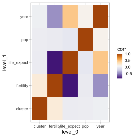
If we were to map a variable that has a natural midpoint, such as a correlation that is defined from -1 to 1, it is not that helpful to use the default colormap, since it will make values close to zero seem more important than value close to -1.
corr_df = data.gapminder().corr().stack().reset_index(name='corr')
alt.Chart(corr_df).mark_rect().encode(
    x='level_0',
    y='level_1',
    tooltip='corr',
    color=alt.Color('corr')).properties(width=200, height=200)
<VegaLite 4 object>

If you see this message, it means the renderer has not been properly enabled
for the frontend that you are using. For more information, see
https://altair-viz.github.io/user_guide/troubleshooting.html
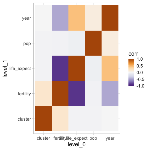
Instead we can choose a color scheme
that is more suitable for showing diverging values,
and define the color domain manually
to match the range of our variable.
An alternative to setting the color scheme explicitly
would have been to set domainMid=0,
in which case Altair understand this is a diverging variable
with a natural midpoint and uses the default diverging color scheme.
(alt.Chart(corr_df).mark_rect().encode(
    x='level_0',
    y='level_1',
    tooltip='corr',
    color=alt.Color('corr', scale=alt.Scale(domain=(-1, 1), scheme='purpleorange')))
 .properties(width=200, height=200))
<VegaLite 4 object>

If you see this message, it means the renderer has not been properly enabled
for the frontend that you are using. For more information, see
https://altair-viz.github.io/user_guide/troubleshooting.html
ggplot#
Categorical#
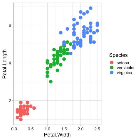
The default categorical colormap in ggplot is not explicitly designed, but rather created by selecting equally spaced colors from the color wheel.
%%R

options(tidyverse.quiet = TRUE)
library(tidyverse)

theme_set(theme_light(base_size = 18))
R[write to console]: Error in (function (filename = "Rplot%03d.png", width = 480, height = 480,  :
  Graphics API version mismatch
---------------------------------------------------------------------------
RRuntimeError                             Traceback (most recent call last)
Input In [11], in <cell line: 1>()
----> 1 get_ipython().run_cell_magic('R', '', '\noptions(tidyverse.quiet = TRUE) \nlibrary(tidyverse)\n\ntheme_set(theme_light(base_size = 18))\n')

File /opt/hostedtoolcache/Python/3.9.13/x64/lib/python3.9/site-packages/IPython/core/interactiveshell.py:2358, in InteractiveShell.run_cell_magic(self, magic_name, line, cell)
   2356 with self.builtin_trap:
   2357     args = (magic_arg_s, cell)
-> 2358     result = fn(*args, **kwargs)
   2359 return result

File /opt/hostedtoolcache/Python/3.9.13/x64/lib/python3.9/site-packages/rpy2/ipython/rmagic.py:765, in RMagics.R(self, line, cell, local_ns)
    762 else:
    763     cell_display = CELL_DISPLAY_DEFAULT
--> 765 tmpd = self.setup_graphics(args)
    767 text_output = ''
    768 try:

File /opt/hostedtoolcache/Python/3.9.13/x64/lib/python3.9/site-packages/rpy2/ipython/rmagic.py:461, in RMagics.setup_graphics(self, args)
    457 tmpd_fix_slashes = tmpd.replace('\\', '/')
    459 if self.device == 'png':
    460     # Note: that %% is to pass into R for interpolation there
--> 461     grdevices.png("%s/Rplots%%03d.png" % tmpd_fix_slashes,
    462                   **argdict)
    463 elif self.device == 'svg':
    464     self.cairo.CairoSVG("%s/Rplot.svg" % tmpd_fix_slashes,
    465                         **argdict)

File /opt/hostedtoolcache/Python/3.9.13/x64/lib/python3.9/site-packages/rpy2/robjects/functions.py:203, in SignatureTranslatedFunction.__call__(self, *args, **kwargs)
    201         v = kwargs.pop(k)
    202         kwargs[r_k] = v
--> 203 return (super(SignatureTranslatedFunction, self)
    204         .__call__(*args, **kwargs))

File /opt/hostedtoolcache/Python/3.9.13/x64/lib/python3.9/site-packages/rpy2/robjects/functions.py:126, in Function.__call__(self, *args, **kwargs)
    124     else:
    125         new_kwargs[k] = cv.py2rpy(v)
--> 126 res = super(Function, self).__call__(*new_args, **new_kwargs)
    127 res = cv.rpy2py(res)
    128 return res

File /opt/hostedtoolcache/Python/3.9.13/x64/lib/python3.9/site-packages/rpy2/rinterface_lib/conversion.py:45, in _cdata_res_to_rinterface.<locals>._(*args, **kwargs)
     44 def _(*args, **kwargs):
---> 45     cdata = function(*args, **kwargs)
     46     # TODO: test cdata is of the expected CType
     47     return _cdata_to_rinterface(cdata)

File /opt/hostedtoolcache/Python/3.9.13/x64/lib/python3.9/site-packages/rpy2/rinterface.py:813, in SexpClosure.__call__(self, *args, **kwargs)
    806     res = rmemory.protect(
    807         openrlib.rlib.R_tryEval(
    808             call_r,
    809             call_context.__sexp__._cdata,
    810             error_occured)
    811     )
    812     if error_occured[0]:
--> 813         raise embedded.RRuntimeError(_rinterface._geterrmessage())
    814 return res

RRuntimeError: Error in (function (filename = "Rplot%03d.png", width = 480, height = 480,  :
  Graphics API version mismatch
%%R

ggplot(iris) +
    aes(x = Petal.Width,
        y = Petal.Length,
        color = Species) +
    geom_point(size = 5)
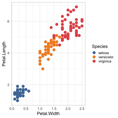
All useful color maps are not collecting in one place,
but available through different functions and packages.
For example,
the color maps from color brewer are accessible via
scale_color|fill_brewer|distiller
(use the brewer suffix for categorical and distiller for sequential values).
ggplot(iris) + aes(x = Petal.Width, y = Petal.Length, color = Species) + geom_point(size = 5) + scale_color_brewer(palette = ‘Dark2’)
All R colors maps can be viewed in this repo. The tableau colors used in Altair are accessible via the ggthemes package.
%%R
ggplot(iris) +
    aes(x = Petal.Width,
        y = Petal.Length,
        color = Species) +
    geom_point(size = 5) +
    ggthemes::scale_color_tableau()
We could also set the colorscale manually, let’s use the same colors as in the altair example, but this time via their HTML codes instead.
%%R
ggplot(iris) +
    aes(x = Petal.Width,
        y = Petal.Length,
        color = Species) +
    geom_point(size = 5) +
    scale_color_manual(values = c('#FF7F50', '#4682B4', '#663399'))

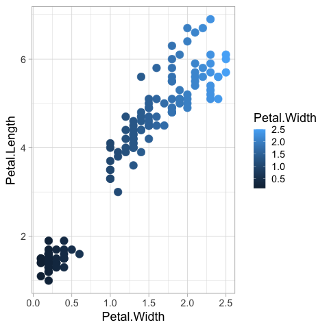
Sequential#
The default color map for numerical values goes from dark to white, since the default background is dark.
%%R
ggplot(iris) +
    aes(x = Petal.Width,
        y = Petal.Length,
        color = Petal.Width) +
    geom_point(size = 5)
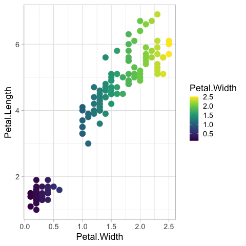
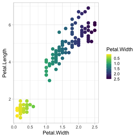
It can be changed to the viridis color map.
%%R
ggplot(iris) +
    aes(x = Petal.Width,
        y = Petal.Length,
        color = Petal.Width) +
    geom_point(size = 5) +
    scale_color_viridis_c()
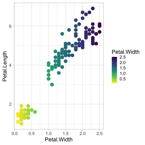
Reversing is possible via the same techniques as for axes, but it does not look great since the color legend is sorted “upside down”.
%%R
ggplot(iris) +
    aes(x = Petal.Width,
        y = Petal.Length,
        color = Petal.Width) +
    geom_point(size = 5) +
    scale_color_viridis_c(trans = 'reverse')
There is a special syntax for colormaps that preserves the orientation of the legend while reversing.
%%R
ggplot(iris) +
    aes(x = Petal.Width,
        y = Petal.Length,
        color = Petal.Width) +
    geom_point(size = 5) +
    scale_color_viridis_c(direction = -1)
Diverging#
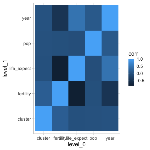
Like in Altair, it is not that informative to use the default color map for diverging values.
%%R -i corr_df
library(tidyverse)

ggplot(corr_df) +
    aes(x = level_0,
        y = level_1,
        fill = corr) +
    geom_tile()
The default bluered tableau diverging color map can be used via ggthemes.
%%R -i corr_df
ggplot(corr_df) +
    aes(x = level_0,
        y = level_1,
        fill = corr) +
    geom_tile() +
    ggthemes::scale_fill_gradient2_tableau()
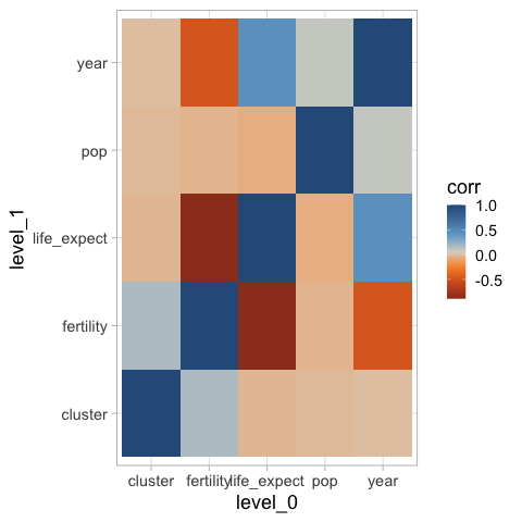
However, this sets blue as high values by default, which is against people’s intuition since red is often used for “hot” and blue or “cold”. We can either reverse the colormap, or use one from ColorBrewer instead.
%%R -i corr_df
ggplot(corr_df) +
    aes(x = level_0,
        y = level_1,
        fill = corr) +
    geom_tile() +
    scale_fill_distiller(palette = 'PuOr')
Defining the colormap limits ensures that low and high values of the same magnitude are equally highlighted.
%%R -i corr_df
ggplot(corr_df) +
    aes(x = level_0,
        y = level_1,
        fill = corr) +
    geom_tile() +
    scale_fill_distiller(palette = 'PuOr', limits = c(-1, 1))
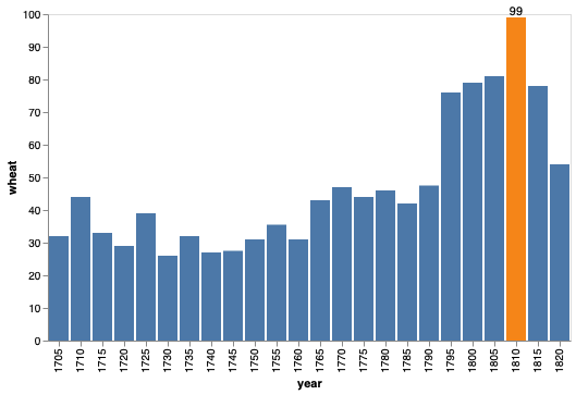
Highlighting with colors and text labels#
We can also use color to highlight manually select elements in plots, for example the year with the highest wheat price in the figure below.
wheat = data.wheat().query('year > 1700')  # Reduce the number of bars for clarity

# Set the year to be highlighted to a separate value in a new column
wheat['highlight'] = False
wheat.loc[wheat['year'] == wheat['year'].iloc[wheat['wages'].argmax()], 'highlight'] = True

alt.Chart(wheat).mark_bar().encode(
    x='year:O',
    y="wheat",
    color='highlight')
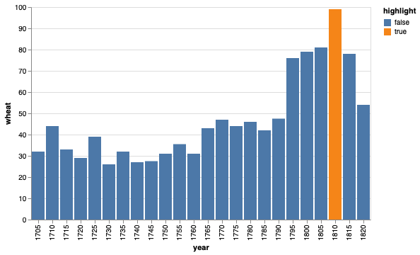
The legend is not that useful here so lets remove it.
alt.Chart(wheat).mark_bar().encode(
    x='year:O',
    y="wheat",
    color=alt.Color('highlight', legend=None))

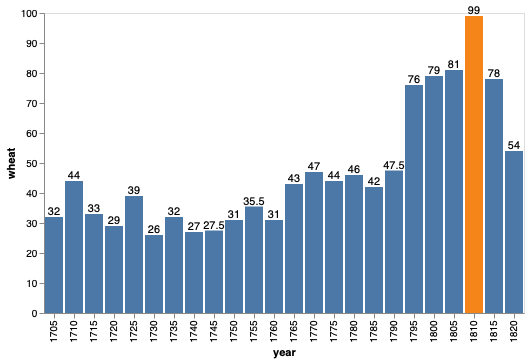
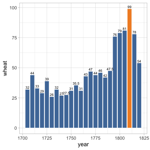
Adding an annotation in the form of the exact price can be helpful.
bars = alt.Chart(wheat).mark_bar().encode(
    x='year:O',
    y="wheat",
    color=alt.Color('highlight', legend=None))
bars + bars.mark_text(dy=-5).encode(text='wheat')

If we want to override the color,
we need to set it in the encoding.
Setting it in the mark would not work
since we are building off a chart which has the encoding color set,
and this has higher precedence than color set in the mark.
To pass a literal value in the encoding
(instead of asking altair to look for a column with this name in the dataframe),
we can use alt.value().
bars = alt.Chart(wheat).mark_bar().encode(
    x='year:O',
    y="wheat",
    color=alt.Color('highlight', legend=None))
bars + bars.mark_text(dy=-5).encode(text='wheat', color=alt.value('black'))

Now that we are supplying the exact value, we no longer need the gridlines, which are there to help infer values (and also make exact comparisons between graphical elements far away from each other).
bars = alt.Chart(wheat).mark_bar().encode(
    x='year:O',
    y=alt.Y('wheat', axis=alt.Axis(grid=False)),
    color=alt.Color('highlight', legend=None))
bars + bars.mark_text(dy=-5).encode(text='wheat', color=alt.value('black'))
Generally, having an outline of a plot is not that aesthetically pleasing. It works well in altair when we have the gridlines since they melt together, but now that they are gone, let’s also remove the outline.
bars = alt.Chart(wheat).mark_bar().encode(
    x='year:O',
    y=alt.Y('wheat', axis=alt.Axis(grid=False)),
    color=alt.Color('highlight', legend=None))
(bars + bars.mark_text(dy=-5).encode(text='wheat', color=alt.value('black'))).configure_view(strokeWidth=0)

We can highlight only the year by filtering the data frame.
bars + alt.Chart(wheat.query('year == 1810')).mark_text(dy=-5).encode(
    x='year:O',
    y=alt.Y("wheat",axis=alt.Axis(grid=False)),
    text='wheat')
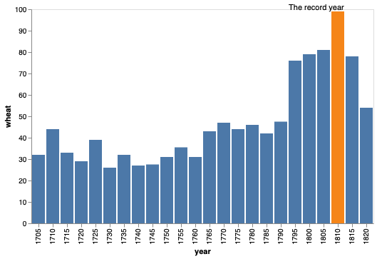
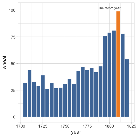
To set a custom text,
we can use alt.value again.
bars + alt.Chart(wheat.query('year == 1810')).mark_text(dy=-5, dx=-30).encode(
    x='year:O',
    y="wheat",
    text=alt.value('The record year'))
To set multiple values, we could either add an annotation column to our existing data frame, or create a new dataframe as below.
import pandas as pd

annot_wheat = pd.DataFrame({'year': [1730, 1810], 'wheat': [26, 99], 'text': ['The lowest year', 'The record year']})
annot_wheat
| year | wheat | text | |
|---|---|---|---|
| 0 | 1730 | 26 | The lowest year |
| 1 | 1810 | 99 | The record year |
bars + alt.Chart(annot_wheat).mark_text(dy=-5).encode(
    x='year:O',
    y="wheat",
    text='text')

To avoid the overlap of the new annotation and the blue bars,
we would have to create the annotations in two separate steps
and change their text position or color accordingly.
If using two separate steps,
we can also use the alt.value() technique,
which avoids us having to create the new data frame.
ggplot#
Using the dataframe with the highlight column, we can set the fill accordingly.
%%R -i wheat
ggplot(wheat) +
    aes(x = year,
        y = wheat,
        fill = highlight) +
    geom_bar(stat = 'identity', color = 'white') +
    ggthemes::scale_fill_tableau()
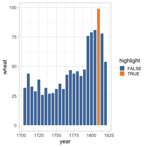
And remove the legend.
%%R
ggplot(wheat) +
    aes(x = year,
        y = wheat,
        fill = highlight) +
    geom_bar(stat = 'identity', color = 'white') +
    ggthemes::scale_fill_tableau() +
    theme(legend.position = 'none')
To add annotations,
we can use geom_text
with the label aesthetic.
%%R
ggplot(wheat) +
    aes(x = year,
        y = wheat,
        fill = highlight,
        label = wheat) +
    geom_bar(stat = 'identity', color = 'white') +
    geom_text(vjust=-0.3) +
    ggthemes::scale_fill_tableau() +
    theme(legend.position = 'none')
To get these to be the same colors as the bars,
we can set the color aestethic,
and add the corresponding color scale.
%%R
ggplot(wheat) +
    aes(x = year,
        y = wheat,
        fill = highlight,
        label = wheat,
        color = highlight) +
    geom_bar(stat = 'identity', color = 'white') +
    geom_text(vjust=-0.3) +
    ggthemes::scale_fill_tableau() +
    ggthemes::scale_color_tableau() +
    theme(legend.position = 'none')

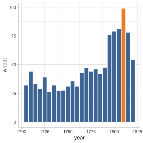
Now we can remove the gridlines.
%%R
ggplot(wheat) +
    aes(x = year,
        y = wheat,
        fill = highlight,
        label = wheat,
        color = highlight) +
    geom_bar(stat = 'identity', color = 'white') +
    geom_text(vjust=-0.3) +
    ggthemes::scale_fill_tableau() +
    ggthemes::scale_color_tableau() +
    theme(legend.position = 'none',
          panel.grid.major = element_blank(),
          panel.grid.minor = element_blank())

If you want your label to represent the count
(which we normally calculate in the geom for ggplot),
you can set it to label = stat(count).
To set a specific annotation text,
we could either use the same approach as in Altair
of adding a new column to our data frame,
or we could use the annotate function.
%%R
ggplot(wheat) +
    aes(x = year,
        y = wheat,
        fill = highlight) +
    geom_bar(stat = 'identity', color = 'white') +
    annotate('text', label = 'The record year', x = 1800, y = 102) +
    ggthemes::scale_fill_tableau() +
    theme(legend.position = 'none')
Direct labeling instead of using a legend#
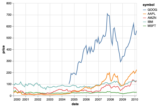
In the example below, the legend is not in the same order as where the lines end, which can make it a bit less intuitive to read.
stocks = data.stocks()

alt.Chart(stocks).mark_line().encode(
    x='date',
    y='price',
    color='symbol')

We can align the ordering of these two,
by calculating the order of the lines at the maximum year
and then and then passing the labels in this order as a list to the sort parameter.
stock_order = (
    stocks
    .loc[stocks['date'] == stocks['date'].max()]
    .sort_values('price', ascending=False))
stock_order
| symbol | date | price | |
|---|---|---|---|
| 436 | GOOG | 2010-03-01 | 560.19 |
| 559 | AAPL | 2010-03-01 | 223.02 |
| 245 | AMZN | 2010-03-01 | 128.82 |
| 368 | IBM | 2010-03-01 | 125.55 |
| 122 | MSFT | 2010-03-01 | 28.80 |
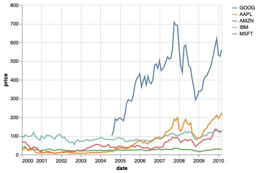
alt.Chart(stocks).mark_line().encode(
    x='date',
    y='price',
    color=alt.Color('symbol', sort=stock_order['symbol'].tolist()))
The title for categorical axes or legends are often not that informative, and in many cases we can remove it.
alt.Chart(stocks).mark_line().encode(
    x='date',
    y='price',
    color=alt.Color(
        'symbol',
        sort=stock_order['symbol'].tolist(),
        legend=alt.Legend(title=None)))
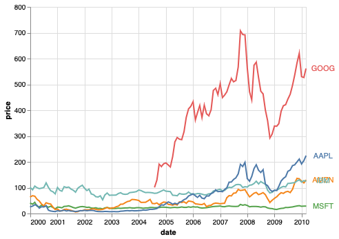
We can use the annotation approach from above to label the lines directly, and get rid of the legend altogether.
lines = alt.Chart(stocks).mark_line().encode(
    x='date',
    y='price',
    color=alt.Color('symbol', legend=None))

text = alt.Chart(stock_order).mark_text(dx=25).encode(
    x='date',
    y='price',
    text='symbol',
    color='symbol')

lines + text
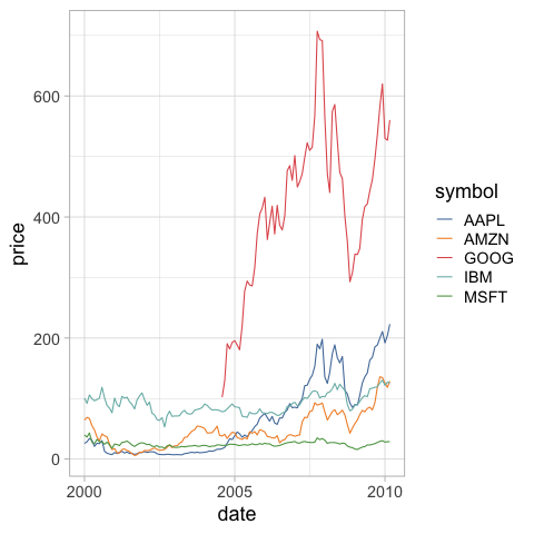
ggplot#
%%R -i stocks
ggplot(stocks) +
    aes(x = date,
        y = price,
        color = symbol) +
    geom_line() +
    ggthemes::scale_color_tableau()
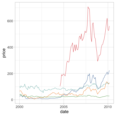
%%R
ggplot(stocks) +
    aes(x = date,
        y = price,
        color = symbol) +
    geom_line() +
    ggthemes::scale_color_tableau() +
    theme(legend.position = 'none')
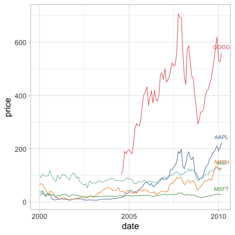
Here we use the same approach with geom_text and label as we did above.
The difference is that we’re explicitly setting the data inside geom_text
to use the dataframe that has been filtered to contain the max year only.
%%R -i stock_order
ggplot(stocks) +
    aes(x = date,
        y = price,
        color = symbol,
        label = symbol) +
    geom_line() +
    geom_text(data = stock_order, vjust=-1) +
    ggthemes::scale_color_tableau() +
    theme(legend.position = 'none')
You can try the ggrepel package to help you with annotations. It’s pretty cool!
%%R -i stock_order
library(ggrepel())

extrema <-
  stocks %>%
    group_by(symbol) %>%
    slice(which.max(date))

# Adding a couple of years to the date
extrema['date'] = extrema['date'] + 5E7

ggplot(stocks) +
    aes(x = date,
        y = price,
        color = symbol,
        label = symbol) +
    geom_line() +
    ggthemes::scale_color_tableau() +
    geom_text_repel(
        data = extrema,
        aes(date, label = symbol),
        min.segment.length = Inf,
      )
R[write to console]: Error in library(ggrepel()) : there is no package called ‘ggrepel’
Error in library(ggrepel()) : there is no package called ‘ggrepel’
---------------------------------------------------------------------------
RRuntimeError                             Traceback (most recent call last)
~/.pyenv/versions/3.9.7/lib/python3.9/site-packages/rpy2/ipython/rmagic.py in eval(self, code)
    267                 # Need the newline in case the last line in code is a comment.
--> 268                 value, visible = ro.r("withVisible({%s\n})" % code)
    269             except (ri.embedded.RRuntimeError, ValueError) as exception:

~/.pyenv/versions/3.9.7/lib/python3.9/site-packages/rpy2/robjects/__init__.py in __call__(self, string)
    437         p = rinterface.parse(string)
--> 438         res = self.eval(p)
    439         return conversion.rpy2py(res)

~/.pyenv/versions/3.9.7/lib/python3.9/site-packages/rpy2/robjects/functions.py in __call__(self, *args, **kwargs)
    197                 kwargs[r_k] = v
--> 198         return (super(SignatureTranslatedFunction, self)
    199                 .__call__(*args, **kwargs))

~/.pyenv/versions/3.9.7/lib/python3.9/site-packages/rpy2/robjects/functions.py in __call__(self, *args, **kwargs)
    124                 new_kwargs[k] = conversion.py2rpy(v)
--> 125         res = super(Function, self).__call__(*new_args, **new_kwargs)
    126         res = conversion.rpy2py(res)

~/.pyenv/versions/3.9.7/lib/python3.9/site-packages/rpy2/rinterface_lib/conversion.py in _(*args, **kwargs)
     44     def _(*args, **kwargs):
---> 45         cdata = function(*args, **kwargs)
     46         # TODO: test cdata is of the expected CType

~/.pyenv/versions/3.9.7/lib/python3.9/site-packages/rpy2/rinterface.py in __call__(self, *args, **kwargs)
    679             if error_occured[0]:
--> 680                 raise embedded.RRuntimeError(_rinterface._geterrmessage())
    681         return res

RRuntimeError: Error in library(ggrepel()) : there is no package called ‘ggrepel’


During handling of the above exception, another exception occurred:

RInterpreterError                         Traceback (most recent call last)
/var/folders/64/bfv2dn992m17r4ztvfrt93rh0000gn/T/ipykernel_57633/2631548253.py in <module>
----> 1 get_ipython().run_cell_magic('R', '-i stock_order', "library(ggrepel())\n\nextrema <- \n  stocks %>%\n    group_by(symbol) %>%\n    slice(which.max(date))\n\n# Adding a couple of years to the date\nextrema['date'] = extrema['date'] + 5E7\n\nggplot(stocks) + \n    aes(x = date,\n        y = price,\n        color = symbol,\n        label = symbol) +\n    geom_line() +\n    ggthemes::scale_color_tableau() +\n    geom_text_repel(\n        data = extrema,\n        aes(date, label = symbol),\n        min.segment.length = Inf,\n      )\n")

~/.pyenv/versions/3.9.7/lib/python3.9/site-packages/IPython/core/interactiveshell.py in run_cell_magic(self, magic_name, line, cell)
   2401             with self.builtin_trap:
   2402                 args = (magic_arg_s, cell)
-> 2403                 result = fn(*args, **kwargs)
   2404             return result
   2405

~/.pyenv/versions/3.9.7/lib/python3.9/site-packages/decorator.py in fun(*args, **kw)
    230             if not kwsyntax:
    231                 args, kw = fix(args, kw, sig)
--> 232             return caller(func, *(extras + args), **kw)
    233     fun.__name__ = func.__name__
    234     fun.__doc__ = func.__doc__

~/.pyenv/versions/3.9.7/lib/python3.9/site-packages/IPython/core/magic.py in <lambda>(f, *a, **k)
    185     # but it's overkill for just that one bit of state.
    186     def magic_deco(arg):
--> 187         call = lambda f, *a, **k: f(*a, **k)
    188
    189         if callable(arg):

~/.pyenv/versions/3.9.7/lib/python3.9/site-packages/rpy2/ipython/rmagic.py in R(self, line, cell, local_ns)
    781             if not e.stdout.endswith(e.err):
    782                 print(e.err)
--> 783             raise e
    784         finally:
    785             if self.device in ['png', 'svg']:

~/.pyenv/versions/3.9.7/lib/python3.9/site-packages/rpy2/ipython/rmagic.py in R(self, line, cell, local_ns)
    761                     return_output = False
    762             else:
--> 763                 text_result, result, visible = self.eval(code)
    764                 text_output += text_result
    765                 if visible:

~/.pyenv/versions/3.9.7/lib/python3.9/site-packages/rpy2/ipython/rmagic.py in eval(self, code)
    270                 # Otherwise next return seems to have copy of error.
    271                 warning_or_other_msg = self.flush()
--> 272                 raise RInterpreterError(code, str(exception),
    273                                         warning_or_other_msg)
    274             text_output = self.flush()

RInterpreterError: Failed to parse and evaluate line "library(ggrepel())\n\nextrema <- \n  stocks %>%\n    group_by(symbol) %>%\n    slice(which.max(date))\n\n# Adding a couple of years to the date\nextrema['date'] = extrema['date'] + 5E7\n\nggplot(stocks) + \n    aes(x = date,\n        y = price,\n        color = symbol,\n        label = symbol) +\n    geom_line() +\n    ggthemes::scale_color_tableau() +\n    geom_text_repel(\n        data = extrema,\n        aes(date, label = symbol),\n        min.segment.length = Inf,\n      )\n".
R error message: 'Error in library(ggrepel()) : there is no package called ‘ggrepel’'