Lecture 5 - Tidy control flow in R#

Lecture learning objectives:#

By the end of this lecture and worksheet 5, students should be able to:

Explain what a grouped data frame is, and how it can be used
Use {dplyr}’s group_by + summarize to perform the split-apply-combine approach in R to iterate over and summarize data by groups
Identify missing and erroneous values and manage them by removing (via {dplyr}’s filter) or replacing (using {dplyr}’s mutate + case_when)
Identify where in R code a commonly used functional, a {purrr}’s map* function, could be used in place of for loops and write code to do this

library(gapminder)
library(tidyverse)
options(repr.matrix.max.rows = 10)

Error in library(gapminder): there is no package called ‘gapminder’
Traceback:

1. library(gapminder)

Change or remove specific values#

Sometimes we’d like to selectively change values, we can do this using control flow within mutate
A related task is removing rows where there are NAs, either in a specified column or across the whole data frame or tibble

Selectively change a values#

What if we want to programatically change certain values? For example, update the country name “Cambodia” to its official English name, “Kingdom of Cambodia”?

If we want to change one or more (but not all things) in a column, one function we can use is case_when inside a mutate call:

gapminder %>% 
    mutate(country = case_when(country == "Cambodia" ~ "Kingdom of Cambodia",
                            TRUE ~ country))

Error: Problem with `mutate()` input `country`.
✖ must be a character vector, not a `factor` object.
ℹ Input `country` is `case_when(...)`.
Traceback:

1. gapminder %>% mutate(country = case_when(country == "Cambodia" ~ 
 .     "Kingdom of Cambodia", TRUE ~ country))
2. withVisible(eval(quote(`_fseq`(`_lhs`)), env, env))
3. eval(quote(`_fseq`(`_lhs`)), env, env)
4. eval(quote(`_fseq`(`_lhs`)), env
...

Ah! This doesn’t work? What is going on here? Let’s look at the structure of gapminder:

str(gapminder)

tibble [1,704 × 6] (S3: tbl_df/tbl/data.frame)
 $ country  : Factor w/ 142 levels "Afghanistan",..: 1 1 1 1 1 1 1 1 1 1 ...
 $ continent: Factor w/ 5 levels "Africa","Americas",..: 3 3 3 3 3 3 3 3 3 3 ...
 $ year     : int [1:1704] 1952 1957 1962 1967 1972 1977 1982 1987 1992 1997 ...
 $ lifeExp  : num [1:1704] 28.8 30.3 32 34 36.1 ...
 $ pop      : int [1:1704] 8425333 9240934 10267083 11537966 13079460 14880372 12881816 13867957 16317921 22227415 ...
 $ gdpPercap: num [1:1704] 779 821 853 836 740 ...

country (and continent) are factors! Let’s change these to character vectors so we can manipulate the character values they hold. We’ll make a new tibble named gap to do this:

gap <- gapminder %>% 
    mutate(country = as.character(country),
          continent = as.character(continent))

OK, now let’s try that conditional mutate again!

gap <- gap %>% 
    mutate(country = case_when(country == "Cambodia" ~ "Kingdom of Cambodia",
                            TRUE ~ country))
gap

A tibble: 1704 × 6
country	continent	year	lifeExp	pop	gdpPercap
<chr>	<chr>	<int>	<dbl>	<int>	<dbl>
Afghanistan	Asia	1952	28.801	8425333	779.4453
Afghanistan	Asia	1957	30.332	9240934	820.8530
Afghanistan	Asia	1962	31.997	10267083	853.1007
Afghanistan	Asia	1967	34.020	11537966	836.1971
Afghanistan	Asia	1972	36.088	13079460	739.9811
⋮	⋮	⋮	⋮	⋮	⋮
Zimbabwe	Africa	1987	62.351	9216418	706.1573
Zimbabwe	Africa	1992	60.377	10704340	693.4208
Zimbabwe	Africa	1997	46.809	11404948	792.4500
Zimbabwe	Africa	2002	39.989	11926563	672.0386
Zimbabwe	Africa	2007	43.487	12311143	469.7093

Did it work?

gap %>%
    filter(country == "Kingdom of Cambodia")

A tibble: 12 × 6
country	continent	year	lifeExp	pop	gdpPercap
<chr>	<chr>	<int>	<dbl>	<int>	<dbl>
Kingdom of Cambodia	Asia	1952	39.417	4693836	368.4693
Kingdom of Cambodia	Asia	1957	41.366	5322536	434.0383
Kingdom of Cambodia	Asia	1962	43.415	6083619	496.9136
Kingdom of Cambodia	Asia	1967	45.415	6960067	523.4323
Kingdom of Cambodia	Asia	1972	40.317	7450606	421.6240
⋮	⋮	⋮	⋮	⋮	⋮
Kingdom of Cambodia	Asia	1987	53.914	8371791	683.8956
Kingdom of Cambodia	Asia	1992	55.803	10150094	682.3032
Kingdom of Cambodia	Asia	1997	56.534	11782962	734.2852
Kingdom of Cambodia	Asia	2002	56.752	12926707	896.2260
Kingdom of Cambodia	Asia	2007	59.723	14131858	1713.7787

Selectively change two or more values with `case_when`#

case_when will also let us easily modify > 2 cases. What if, for example, we wanted to change the continents from their English name to their French name?

french_contients <- gap %>% 
  mutate(continent = case_when(continent == "Asia" ~ "Asie", 
                               continent == "Europe" ~ "L'Europe",
                               continent == "Africa" ~ "Afrique", 
                               continent == "Americas" ~ "les amériques", 
                               continent == "Oceania" ~ "Océanie"))
head(french_contients)

A tibble: 6 × 6
country	continent	year	lifeExp	pop	gdpPercap
<chr>	<chr>	<int>	<dbl>	<int>	<dbl>
Afghanistan	Asie	1952	28.801	8425333	779.4453
Afghanistan	Asie	1957	30.332	9240934	820.8530
Afghanistan	Asie	1962	31.997	10267083	853.1007
Afghanistan	Asie	1967	34.020	11537966	836.1971
Afghanistan	Asie	1972	36.088	13079460	739.9811
Afghanistan	Asie	1977	38.438	14880372	786.1134

What if we don’t want to change Asia?

french_contients <- gap %>% 
  mutate(continent = case_when(#continent == "Asia" ~ "Asie", 
                               continent == "Europe" ~ "L'Europe",
                               continent == "Africa" ~ "Afrique", 
                               continent == "Americas" ~ "les amériques", 
                               continent == "Oceania" ~ "Océanie"))
head(french_contients)

A tibble: 6 × 6
country	continent	year	lifeExp	pop	gdpPercap
<chr>	<chr>	<int>	<dbl>	<int>	<dbl>
Afghanistan	NA	1952	28.801	8425333	779.4453
Afghanistan	NA	1957	30.332	9240934	820.8530
Afghanistan	NA	1962	31.997	10267083	853.1007
Afghanistan	NA	1967	34.020	11537966	836.1971
Afghanistan	NA	1972	36.088	13079460	739.9811
Afghanistan	NA	1977	38.438	14880372	786.1134

Uh oh, now Asia is NA?? We need to say TRUE ~ column_name to tell R to not put in NA’s in the non-specified class, but instead leave the values that were already there:

french_contients <- gap %>% 
  mutate(continent = case_when(#continent == "Asia" ~ "Asie", 
                               continent == "Europe" ~ "L'Europe",
                               continent == "Africa" ~ "Afrique", 
                               continent == "Americas" ~ "les amériques", 
                               continent == "Oceania" ~ "Océanie", 
                               TRUE ~ continent))
head(french_contients)

A tibble: 6 × 6
country	continent	year	lifeExp	pop	gdpPercap
<chr>	<chr>	<int>	<dbl>	<int>	<dbl>
Afghanistan	Asia	1952	28.801	8425333	779.4453
Afghanistan	Asia	1957	30.332	9240934	820.8530
Afghanistan	Asia	1962	31.997	10267083	853.1007
Afghanistan	Asia	1967	34.020	11537966	836.1971
Afghanistan	Asia	1972	36.088	13079460	739.9811
Afghanistan	Asia	1977	38.438	14880372	786.1134

Removing rows where a specific column holds NAs#

Here, we’d like to remove the rows where the column x is NA:

df <- tibble(x = c(3, 1, 2, NA), y = c("z", "a", NA, "b"))
df

A tibble: 4 × 2
x	y
<dbl>	<chr>
3	z
1	a
2	NA
NA	b

drop_na is the tidyverse function we can use to do this.

In this case we pass the column for which we would like to use to drive the removal of rows (based on the presence of NAs in that row):

df %>% drop_na(x:y)

A tibble: 2 × 2
x	y
<dbl>	<chr>
3	z
1	a

Removing all rows where there is a NA in any column#

If no arguments are given to drop_na, then all rows with NAs will be dropped:

df %>% drop_na()

A tibble: 2 × 2
x	y
<dbl>	<chr>
3	z
1	a

Iterate over groups of rows#

`summarise` calculates summaries over rows#

Examples might be calculating the mean horsepower and mean miles per gallon of cars in the mtcars data set:

# calculate mean hp and mpg for all cars
mtcars %>% 
    summarise(mean_hp = mean(hp),
             mean_mpg = mean(mpg),
             sum_hp = sum(hp))

A data.frame: 1 × 3
mean_hp	mean_mpg	sum_hp
<dbl>	<dbl>	<dbl>
146.6875	20.09062	4694

Iteration with `group_by` + `summarise`#

Useful when you want to do something repeatedly to a group of rows
An example, say we want to calculate the average life expectancy (lifeExp) for each continent from the gapminder data set

# calculate the average life expectancy for each continent
gapminder %>% 
    group_by(continent) %>% 
    summarise(mean_life_exp = mean(lifeExp))

A tibble: 5 × 2
continent	mean_life_exp
<fct>	<dbl>
Africa	48.86533
Americas	64.65874
Asia	60.06490
Europe	71.90369
Oceania	74.32621

We can also group_by multiple columns, for example what if we want to know the mean life expectancy for each continent and each year:

# calculate the mean life expectancy for each continent and each year
gapminder %>% 
    group_by(continent, year) %>% 
    summarise(mean_life_exp = mean(lifeExp))

`summarise()` has grouped output by 'continent'. You can override using the `.groups` argument.

A grouped_df: 60 × 3
continent	year	mean_life_exp
<fct>	<int>	<dbl>
Africa	1952	39.13550
Africa	1957	41.26635
Africa	1962	43.31944
Africa	1967	45.33454
Africa	1972	47.45094
⋮	⋮	⋮
Oceania	1987	75.3200
Oceania	1992	76.9450
Oceania	1997	78.1900
Oceania	2002	79.7400
Oceania	2007	80.7195

Watch those NA’s!#

Calculate the maximum beak length for each of the Penguin species in the {palmerpenguins} penguins dataset.

library(palmerpenguins)
penguins

A tibble: 344 × 8
species	island	bill_length_mm	bill_depth_mm	flipper_length_mm	body_mass_g	sex	year
<fct>	<fct>	<dbl>	<dbl>	<int>	<int>	<fct>	<int>
Adelie	Torgersen	39.1	18.7	181	3750	male	2007
Adelie	Torgersen	39.5	17.4	186	3800	female	2007
Adelie	Torgersen	40.3	18.0	195	3250	female	2007
Adelie	Torgersen	NA	NA	NA	NA	NA	2007
Adelie	Torgersen	36.7	19.3	193	3450	female	2007
⋮	⋮	⋮	⋮	⋮	⋮	⋮	⋮
Chinstrap	Dream	55.8	19.8	207	4000	male	2009
Chinstrap	Dream	43.5	18.1	202	3400	female	2009
Chinstrap	Dream	49.6	18.2	193	3775	male	2009
Chinstrap	Dream	50.8	19.0	210	4100	male	2009
Chinstrap	Dream	50.2	18.7	198	3775	female	2009

penguins %>%
    group_by(species) %>%
    summarise(max_bill_length = max(bill_length_mm))

A tibble: 3 × 2
species	max_bill_length
<fct>	<dbl>
Adelie	NA
Chinstrap	58
Gentoo	NA

Huh???

By default, summary statistics functions in R return NA if there are any NA observations in the data… This is often not ideal, what we’d like would be for R to just ignore the NA’s and kindly return us the statistic we asked for. We can specify this by setting the na.rm argument to TRUE.

penguins %>%
    group_by(species) %>%
    summarise(max_bill_length = max(bill_length_mm, na.rm = TRUE))

A tibble: 3 × 2
species	max_bill_length
<fct>	<dbl>
Adelie	46.0
Chinstrap	58.0
Gentoo	59.6

Grouped mutate#

Sometimes you don’t want to collapse the n rows for each group into one row. You want to keep your groups, but compute within them.

Let’s make a new variable that is the years of life expectancy gained (lost) relative to 1952, for each individual country. We group by country and use mutate to make a new variable. The first function extracts the first value from a vector. Notice that first is operating on the vector of life expectancies within each country group.

# calculate life expectancy gained (or lost) relative to 1952
gapminder %>% 
    group_by(country) %>% 
    mutate(life_exp_gain = lifeExp - first(lifeExp)) %>% 
    head()

A grouped_df: 6 × 7
country	continent	year	lifeExp	pop	gdpPercap	life_exp_gain
<fct>	<fct>	<int>	<dbl>	<int>	<dbl>	<dbl>
Afghanistan	Asia	1952	28.801	8425333	779.4453	0.000
Afghanistan	Asia	1957	30.332	9240934	820.8530	1.531
Afghanistan	Asia	1962	31.997	10267083	853.1007	3.196
Afghanistan	Asia	1967	34.020	11537966	836.1971	5.219
Afghanistan	Asia	1972	36.088	13079460	739.9811	7.287
Afghanistan	Asia	1977	38.438	14880372	786.1134	9.637

Purrring instead of for loops#

https://purrr.tidyverse.org/

{purrr} `map_*` functions#

alternative to for loops that help you make less syntax errors

If you have programmed in R before#

purrr is an alternative to “apply” functions

purrr::map() ≈ base::lapply()

Iterating over columns of a data frame#

Say, for example we wanted to calculate the median for each column in the mtcars data frame:

head(mtcars)

A data.frame: 6 × 11
	mpg	cyl	disp	hp	drat	wt	qsec	vs	am	gear	carb
	<dbl>	<dbl>	<dbl>	<dbl>	<dbl>	<dbl>	<dbl>	<dbl>	<dbl>	<dbl>	<dbl>
Mazda RX4	21.0	6	160	110	3.90	2.620	16.46	0	1	4	4
Mazda RX4 Wag	21.0	6	160	110	3.90	2.875	17.02	0	1	4	4
Datsun 710	22.8	4	108	93	3.85	2.320	18.61	1	1	4	1
Hornet 4 Drive	21.4	6	258	110	3.08	3.215	19.44	1	0	3	1
Hornet Sportabout	18.7	8	360	175	3.15	3.440	17.02	0	0	3	2
Valiant	18.1	6	225	105	2.76	3.460	20.22	1	0	3	1

medians <- vector("double", ncol(mtcars))
for (i in seq_along(mtcars)) {
    medians[i] <- median(mtcars[[i]], na.rm = TRUE)
}

OK, then next we want to calculate the mean for all of the columns:

means <- vector("double", ncol(mtcars))
for (i in seq_along(mtcars)) {
    means[i] <- mean(mtcars[[i]], na.rm = TRUE)
}

OK, and then the variance…

variances <- vector("double", ncol(mtcars))
for (i in seq_along(mtcars)) {
    variances[i] <- var(mtcars[[i]], na.rm = TRUE)
}

This is getting a little repetitive… What are we repeating?

Can we write this as a function?#

Given that functions are objects in R, this seems reasonable!

medians <- vector("double", ncol(mtcars))
for (i in seq_along(mtcars)) {
    medians[i] <- median(mtcars[[i]], na.rm = TRUE)
}

This is essentially the guts of purrr::map_dbl. The only difference is that is coded in C and the use of ... for additional arguments.

mds_map <- function(x, fun)  {
    out <- vector("double", ncol(x))
    for (i in seq_along(x)) {
        out[i] <- fun(x[[i]], na.rm = TRUE)
    }
    out
}
mds_map(mtcars, min)

10.4
4
71.1
52
2.76
1.513
14.5
0
0
3
1

Functionals#

We have just written what is called a functional.

A functional is a function that takes a function (and other things) as an input and returns a vector as output.

R has several other functionals outside of purrr that you might have already encountered: lapply, apply, tapply, integrate or optim.

What can you do with functionals?#

Common use is as an alternative to for loops

For loops are actually quite effective for iteration, and efficient when used, however it is easy to make mistakes when setting them up as you have to:
- pre-allocate space for the output
- iterate over the thing the right amount of times
- properly use the iteration index

Of course someone has to write for loops#

It doesn’t have to be you#

– Jenny Bryan, Software Engineer at RStudio and UBC MDS Founder

The `purrr::map*` family of functions#

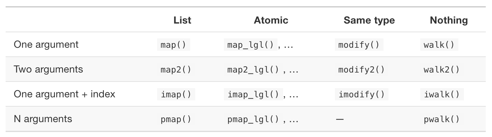
Source: Advanced R by Hadley Wickham

Let’s start at the beginning with the most general `purrr` function: `map`#

map(.x, .f, ...)

Above reads as: for every element of .x apply .f

and can be pictured as:

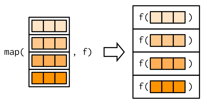
https://d33wubrfki0l68.cloudfront.net/12f6af8404d9723dff9cc665028a35f07759299d/d0d9a/diagrams/functionals/map-list.png

Or picture as…

Source: Row-oriented workflows in R with the tidyverse by Jenny Bryan

Source: Row-oriented workflows in R with the tidyverse by Jenny Bryan

`purrr::map` test drive#

Let’s calculate the median of all the columns of the mtcars data frame using purrr::map:

library(purrr)
map(mtcars, median)

$mpg: 19.2
$cyl: 6
$disp: 196.3
$hp: 123
$drat: 3.695
$wt: 3.325
$qsec: 17.71
$vs: 0
$am: 0
$gear: 4
$carb: 2

That looks different from our mds_map function! The output is of type list. We can use map_df to get a vector of type double:

map_dbl(mtcars, median)

mpg: 19.2
cyl: 6
disp: 196.3
hp: 123
drat: 3.695
wt: 3.325
qsec: 17.71
vs: 0
am: 0
gear: 4
carb: 2

And map_df will give us a tibble:

map_df(mtcars, median)

A tibble: 1 × 11
mpg	cyl	disp	hp	drat	wt	qsec	vs	am	gear	carb
<dbl>	<dbl>	<dbl>	<dbl>	<dbl>	<dbl>	<dbl>	<dbl>	<dbl>	<dbl>	<dbl>
19.2	6	196.3	123	3.695	3.325	17.71	0	0	4	2

So now it’s super efficient and easy to get several summary stats across columns!

map_df(mtcars, median)
map_df(mtcars, mean)
map_df(mtcars, max)
map_df(mtcars, min)

A tibble: 1 × 11
mpg	cyl	disp	hp	drat	wt	qsec	vs	am	gear	carb
<dbl>	<dbl>	<dbl>	<dbl>	<dbl>	<dbl>	<dbl>	<dbl>	<dbl>	<dbl>	<dbl>
19.2	6	196.3	123	3.695	3.325	17.71	0	0	4	2

A tibble: 1 × 11
mpg	cyl	disp	hp	drat	wt	qsec	vs	am	gear	carb
<dbl>	<dbl>	<dbl>	<dbl>	<dbl>	<dbl>	<dbl>	<dbl>	<dbl>	<dbl>	<dbl>
20.09062	6.1875	230.7219	146.6875	3.596563	3.21725	17.84875	0.4375	0.40625	3.6875	2.8125

A tibble: 1 × 11
mpg	cyl	disp	hp	drat	wt	qsec	vs	am	gear	carb
<dbl>	<dbl>	<dbl>	<dbl>	<dbl>	<dbl>	<dbl>	<dbl>	<dbl>	<dbl>	<dbl>
33.9	8	472	335	4.93	5.424	22.9	1	1	5	8

A tibble: 1 × 11
mpg	cyl	disp	hp	drat	wt	qsec	vs	am	gear	carb
<dbl>	<dbl>	<dbl>	<dbl>	<dbl>	<dbl>	<dbl>	<dbl>	<dbl>	<dbl>	<dbl>
10.4	4	71.1	52	2.76	1.513	14.5	0	0	3	1

What if our data frame had missing values?#

Let’s make some to see the consequences…

mtcars_NA <- mtcars
mtcars_NA[1, 1] <- NA

map_dbl(mtcars_NA, median)

mpg: <NA>
cyl: 6
disp: 196.3
hp: 123
drat: 3.695
wt: 3.325
qsec: 17.71
vs: 0
am: 0
gear: 4
carb: 2

How do we tell median to ignore NA’s? Using na.rm = TRUE! But how do we add this to our map_dbl call?

map_dbl(mtcars_NA, median, na.rm = TRUE)

mpg: 19.2
cyl: 6
disp: 196.3
hp: 123
drat: 3.695
wt: 3.325
qsec: 17.71
vs: 0
am: 0
gear: 4
carb: 2

That’s all we will learn of the {purrr} functions for now - however we will meet them again (and learn more about them) next week when we start working with nested data frames.

What did we learn today?#

How to use case_when to selectively change values in a data frame (similar to base R if statements)
How to use group_by to iterate over groups of rows (similar to for loops in base R)
How to use {purrr} map_* functions to iterate over columns (similar to for loops in base R)

Attributions#

Stat 545 created by Jenny Bryan
R for Data Science by Garrett Grolemund & Hadley Wickham

DATA 542

Lecture 5 - Tidy control flow in R

Contents

Lecture 5 - Tidy control flow in R#

Lecture learning objectives:#

Change or remove specific values#

Selectively change a values#

Selectively change two or more values with `case_when`#

Removing rows where a specific column holds NAs#

Removing all rows where there is a NA in any column#

Iterate over groups of rows#

`summarise` calculates summaries over rows#

Iteration with `group_by` + `summarise`#

Watch those NA’s!#

Grouped mutate#

Purrring instead of for loops#

{purrr} `map_*` functions#

If you have programmed in R before#

Iterating over columns of a data frame#

Can we write this as a function?#

Functionals#

What can you do with functionals?#

Of course someone has to write for loops#

It doesn’t have to be you#

The `purrr::map*` family of functions#

Let’s start at the beginning with the most general `purrr` function: `map`#

`purrr::map` test drive#

What if our data frame had missing values?#

What did we learn today?#

Attributions#

DATA 542

Lecture 5 - Tidy control flow in R

Contents

Lecture 5 - Tidy control flow in R#

Lecture learning objectives:#

Change or remove specific values#

Selectively change a values#

Selectively change two or more values with case_when#

Removing rows where a specific column holds NAs#

Removing all rows where there is a NA in any column#

Iterate over groups of rows#

summarise calculates summaries over rows#

Iteration with group_by + summarise#

Watch those NA’s!#

Grouped mutate#

Purrring instead of for loops#

{purrr} map_* functions#

If you have programmed in R before#

Iterating over columns of a data frame#

Can we write this as a function?#

Functionals#

What can you do with functionals?#

Of course someone has to write for loops#

It doesn’t have to be you#

The purrr::map* family of functions#

Let’s start at the beginning with the most general purrr function: map#

purrr::map test drive#

What if our data frame had missing values?#

What did we learn today?#

Attributions#

Selectively change two or more values with `case_when`#

`summarise` calculates summaries over rows#

Iteration with `group_by` + `summarise`#

{purrr} `map_*` functions#

The `purrr::map*` family of functions#

Let’s start at the beginning with the most general `purrr` function: `map`#

`purrr::map` test drive#