Lecture 3 - dates & times, strings, as well as factors

Lecture learning objectives:

By the end of this lecture and worksheet 3, students should be able to:

• Manipulate dates and times using the {lubridate} package

• Be able to modify strings in a data frame using regular expressions and the {stringr} package

• Cast categorical columns in a data frame as factors when appropriate, and manipulate factor levels as needed in preparation for data visualisation and statistical analysis (using base R and {forcats} package functions)

library(tidyverse)
library(gapminder)
options(repr.matrix.max.rows = 10)

Error in library(tidyverse): there is no package called ‘tidyverse’
Traceback:

1. library(tidyverse)

Tibbles versus data frames

You have seen and heard me talk about data frames and tibbles in R, and sometimes I carelessly interchange the terms. Let’s take moment to discuss the difference between the two!

Tibbles are special data frames, with special/extra properties. The two important ones you will care about are:

• In RStudio, tibbles only output the first 10 rows

• When you numerically subset a data frame to 1 column, you get a vector. However, when you numerically subset a tibble you still get a tibble back.

When you create a data frame using base R functions, either via data.frame or one of the base R read.* functions, you get an objects whose class is data frame:

example <- data.frame(a = c(1, 5, 9), b = "z", "a", "t")
example

class(example)

A data.frame: 3 × 4

a	b	X.a.	X.t.
<dbl>	<chr>	<chr>	<chr>
1	z	a	t
5	z	a	t
9	z	a	t

'data.frame'

Tibbles inherit from the data frame class (meaning that have many of the same properties as data frames), but they also have the extra properties I just discussed:

example2 <- tibble(a = c(1, 5, 9), b = "z", "a", "t")
example

class(example2)

A data.frame: 3 × 4

a	b	X.a.	X.t.
<dbl>	<chr>	<chr>	<chr>
1	z	a	t
5	z	a	t
9	z	a	t

1. 'tbl_df'
2. 'tbl'
3. 'data.frame'

Note: there are some tidyverse functions that will coerce a data frame to a tibble, because what the user is asking for is not possible with a data frame. One such example is group_by (which we will learn about next week):

group_by(example, a) %>% 
    class()

1. 'grouped_df'
2. 'tbl_df'
3. 'tbl'
4. 'data.frame'

Rule of thumb: if you want a tibble, it’s on you to know that and express that explicitly with as_tibble() (if it’s a data frame to start out with).

Dates and times

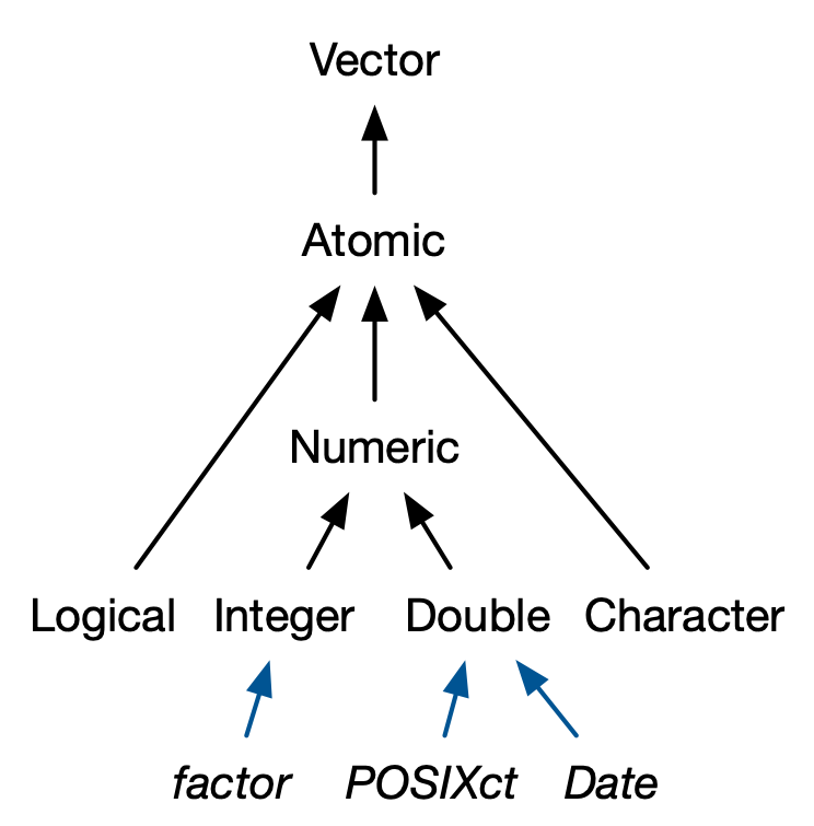
Source: Advanced R by Hadley Wickham

Working with dates and times

Your weapon: The lubridate package (CRAN; GitHub; main vignette).

library(lubridate)

Attaching package: ‘lubridate’


The following objects are masked from ‘package:base’:

    date, intersect, setdiff, union

Get your hands on some dates or date-times

Use lubridate’s today to get today’s date, without any time:

today()

2022-02-01

class(today())

'Date'

Use lubridate’s now to get RIGHT NOW, meaning the date and the time:

now()

[1] "2022-02-01 09:49:35 PST"

class(now())

1. 'POSIXct'
2. 'POSIXt'

Get date or date-time from character

Use the lubridate helpers to convert character or unquoted numbers into dates or date-times:

ymd("2017-01-31")

2017-01-31

mdy("January 31st, 2017")

2017-01-31

dmy("31-Jan-2017")

2017-01-31

ymd(20170131)

2017-01-31

ymd_hms("2017-01-31 20:11:59")

[1] "2017-01-31 20:11:59 UTC"

mdy_hm("01/31/2017 08:01")

[1] "2017-01-31 08:01:00 UTC"

You can also force the creation of a date-time from a date by supplying a timezone:

class(ymd(20170131, tz = "UTC"))

1. 'POSIXct'
2. 'POSIXt'

Build date or date-time from parts

Instead of a single string, sometimes you’ll have the individual components of the date-time spread across multiple columns.

dates <- tibble(year = c(2015, 2016, 2017, 2018, 2019),
               month = c(9, 9, 9, 9, 9),
               day = c(3, 4, 2, 6, 3))

dates

A tibble: 5 × 3

year	month	day
<dbl>	<dbl>	<dbl>
2015	9	3
2016	9	4
2017	9	2
2018	9	6
2019	9	3

To create a date/time from this sort of input, use make_date for dates, or make_datetime for date-times:

# make a single date from year, month and day
dates %>% 
    mutate(date = make_date(year, month, day))

A tibble: 5 × 4

year	month	day	date
<dbl>	<dbl>	<dbl>	<date>
2015	9	3	2015-09-03
2016	9	4	2016-09-04
2017	9	2	2017-09-02
2018	9	6	2018-09-06
2019	9	3	2019-09-03

Getting components from a date or date-time

Sometimes you have the date or date-time and you want to extract a component, such as year or day.

datetime <- ymd_hms("2016-07-08 12:34:56")
datetime

[1] "2016-07-08 12:34:56 UTC"

year(datetime)

2016

month(datetime)

7

mday(datetime)

8

yday(datetime)

190

wday(datetime, label = TRUE, abbr = FALSE)

Friday

Levels:

1. 'Sunday'
2. 'Monday'
3. 'Tuesday'
4. 'Wednesday'
5. 'Thursday'
6. 'Friday'
7. 'Saturday'

For month and wday you can set label = TRUE to return the abbreviated name of the month or day of the week. Set abbr = FALSE to return the full name.

More date and time wrangling possibilities:

• Tools for working with time spans, to calculate durations, periods and intervals

• Tools for dealing with time zones

String manipulations

The recommended tools:

• stringr package: A core package in the tidyverse. Main functions start with str_. Auto-complete is your friend. stringr cheatsheet

• tidyr package: Useful for functions that split one character vector into many and vice versa: separate, unite, extract. tidyr cheatsheet

• Base functions: nchar, strsplit, substr, paste, and paste0.

• The glue package is fantastic for string interpolation. If stringr::str_interp() doesn’t get your job done, check out the glue package.

Regex-free string manipulation with stringr and tidyr

Basic string manipulation tasks:

• Study a single character vector

  • How long are the strings?

  • Presence/absence of a literal string

• Operate on a single character vector

  • Keep/discard elements that contain a literal string

  • Split into two or more character vectors using a fixed delimiter

  • Snip out pieces of the strings based on character position

  • Collapse into a single string

• Operate on two or more character vectors

  • Glue them together element-wise to get a new character vector.

fruit, words, and sentences are character vectors that ship with stringr for practicing.

NOTE - we will be working with vectors today. If you want to operate on data frames, you will need to use these functions inside of data frame/tibble functions, like filter and mutate.

Detect or filter on a target string

Determine presence/absence of a literal string with str_detect. Spoiler: later we see str_detect also detects regular expressions.

Which fruits actually use the word “fruit”?

# detect "fruit"
#typeof(fruit)
#fruit
str_detect(fruit, "fruit")

1. FALSE
2. FALSE
3. FALSE
4. FALSE
5. FALSE
6. FALSE
7. FALSE
8. FALSE
9. FALSE
10. FALSE
11. FALSE
12. TRUE
13. FALSE
14. FALSE
15. FALSE
16. FALSE
17. FALSE
18. FALSE
19. FALSE
20. FALSE
21. FALSE
22. FALSE
23. FALSE
24. FALSE
25. FALSE
26. TRUE
27. FALSE
28. FALSE
29. FALSE
30. FALSE
31. FALSE
32. FALSE
33. FALSE
34. FALSE
35. TRUE
36. FALSE
37. FALSE
38. FALSE
39. TRUE
40. FALSE
41. FALSE
42. TRUE
43. FALSE
44. FALSE
45. FALSE
46. FALSE
47. FALSE
48. FALSE
49. FALSE
50. FALSE
51. FALSE
52. FALSE
53. FALSE
54. FALSE
55. FALSE
56. FALSE
57. TRUE
58. FALSE
59. FALSE
60. FALSE
61. FALSE
62. FALSE
63. FALSE
64. FALSE
65. FALSE
66. FALSE
67. FALSE
68. FALSE
69. FALSE
70. FALSE
71. FALSE
72. FALSE
73. FALSE
74. FALSE
75. TRUE
76. FALSE
77. FALSE
78. FALSE
79. TRUE
80. FALSE

What’s the easiest way to get the actual fruits that match? Use str_subset to keep only the matching elements. Note we are storing this new vector my_fruit to use in later examples!

# subset "fruit"
my_fruit <- str_subset(fruit, "fruit")
my_fruit

1. 'breadfruit'
2. 'dragonfruit'
3. 'grapefruit'
4. 'jackfruit'
5. 'kiwi fruit'
6. 'passionfruit'
7. 'star fruit'
8. 'ugli fruit'

String splitting by delimiter

Use stringr::str_split to split strings on a delimiter.

Some of our fruits are compound words, like “grapefruit”, but some have two words, like “ugli fruit”. Here we split on a single space ” “, but show use of a regular expression later.

# split on " "
str_split(my_fruit, " ")

1. 'breadfruit'
2. 'dragonfruit'
3. 'grapefruit'
4. 'jackfruit'
5. 1. 'kiwi'
   2. 'fruit'
6. 'passionfruit'
7. 1. 'star'
   2. 'fruit'
8. 1. 'ugli'
   2. 'fruit'

It’s bummer that we get a list back. But it must be so! In full generality, split strings must return list, because who knows how many pieces there will be?

If you are willing to commit to the number of pieces, you can use str_split_fixed and get a character matrix. You’re welcome!

str_split_fixed(my_fruit, pattern = " ", n = 2)

A matrix: 8 × 2 of type chr

breadfruit
dragonfruit
grapefruit
jackfruit
kiwi	fruit
passionfruit
star	fruit
ugli	fruit

If the to-be-split variable lives in a data frame, tidyr::separate will split it into 2 or more variables:

# separate on " "
my_fruit[5] <- "yellow kiwi fruit"
my_fruit
tibble(unsplit = my_fruit) %>% 
    separate(unsplit, into = c("pre", "post"), sep = " ")

1. 'breadfruit'
2. 'dragonfruit'
3. 'grapefruit'
4. 'jackfruit'
5. 'yellow kiwi fruit'
6. 'passionfruit'
7. 'star fruit'
8. 'ugli fruit'

Warning message:
“Expected 2 pieces. Additional pieces discarded in 1 rows [5].”
Warning message:
“Expected 2 pieces. Missing pieces filled with `NA` in 5 rows [1, 2, 3, 4, 6].”

A tibble: 8 × 2

pre	post
<chr>	<chr>
breadfruit	NA
dragonfruit	NA
grapefruit	NA
jackfruit	NA
yellow	kiwi
passionfruit	NA
star	fruit
ugli	fruit

Substring extraction (and replacement) by position

Count characters in your strings with str_length. Note this is different from the length of the character vector itself.

# get length of each string
str_length(my_fruit)
my_fruit

1. 10
2. 11
3. 10
4. 9
5. 17
6. 12
7. 10
8. 10

1. 'breadfruit'
2. 'dragonfruit'
3. 'grapefruit'
4. 'jackfruit'
5. 'yellow kiwi fruit'
6. 'passionfruit'
7. 'star fruit'
8. 'ugli fruit'

You can snip out substrings based on character position with str_sub.

# remove first three strings
str_sub(my_fruit, 1, 3)

1. 'bre'
2. 'dra'
3. 'gra'
4. 'jac'
5. 'yel'
6. 'pas'
7. 'sta'
8. 'ugl'

Finally, str_sub also works for assignment, i.e. on the left hand side of <-

# replace three characters with AAA
str_sub(my_fruit, 1, 3)  <- "AAA"
my_fruit

1. 'AAAadfruit'
2. 'AAAgonfruit'
3. 'AAApefruit'
4. 'AAAkfruit'
5. 'AAAlow kiwi fruit'
6. 'AAAsionfruit'
7. 'AAAr fruit'
8. 'AAAi fruit'

Collapse a vector

You can collapse a character vector of length n > 1 to a single string with str_c, which also has other uses (see the next section).

# collapse a character vector into one 
head(fruit) %>% 
    str_c(collapse = "-")

'apple-apricot-avocado-banana-bell pepper-bilberry'

Create a character vector by catenating multiple vectors

If you have two or more character vectors of the same length, you can glue them together element-wise, to get a new vector of that length. Here are some … awful smoothie flavors?

# concatenate character vectors
fruit[1:4]
fruit[5:8]
str_c(fruit[1:4], fruit[5:8], sep = "")

1. 'apple'
2. 'apricot'
3. 'avocado'
4. 'banana'

1. 'bell pepper'
2. 'bilberry'
3. 'blackberry'
4. 'blackcurrant'

1. 'applebell pepper'
2. 'apricotbilberry'
3. 'avocadoblackberry'
4. 'bananablackcurrant'

If the to-be-combined vectors are variables in a data frame, you can use tidyr::unite to make a single new variable from them.

# concatenate character vectors when they are in a data frame
tibble(fruit1 = fruit[1:4],
      fruit2 = fruit[5:8]) %>% 
    unite("flavour_combo", fruit1, fruit2, sep = " & ")

A tibble: 4 × 1

flavour_combo
<chr>
apple & bell pepper
apricot & bilberry
avocado & blackberry
banana & blackcurrant

Substring replacement

You can replace a pattern with str_replace. Here we use an explicit string-to-replace, but later we revisit with a regular expression.

# replace fruit with vegetable
my_fruit <- str_subset(fruit, "fruit")
my_fruit
str_replace(my_fruit, "fruit", "vegetable")

1. 'breadfruit'
2. 'dragonfruit'
3. 'grapefruit'
4. 'jackfruit'
5. 'kiwi fruit'
6. 'passionfruit'
7. 'star fruit'
8. 'ugli fruit'

1. 'breadvegetable'
2. 'dragonvegetable'
3. 'grapevegetable'
4. 'jackvegetable'
5. 'kiwi vegetable'
6. 'passionvegetable'
7. 'star vegetable'
8. 'ugli vegetable'

• A special case that comes up a lot is replacing NA, for which there is str_replace_na.

• If the NA-afflicted variable lives in a data frame, you can use tidyr::replace_na.

Other str_* functions?

There are many many other useful str_* functions from the stringr package. Too many to go through them all here. If these shown in lecture aren’t what you need, then you should try ?str + tab to see the possibilities:

?str_

No documentation for ‘str_’ in specified packages and libraries: you could try ‘??str_’

Regular expressions with stringr

or…

Examples with gapminder

library(gapminder)
head(gapminder)

A tibble: 6 × 6

country	continent	year	lifeExp	pop	gdpPercap
<fct>	<fct>	<int>	<dbl>	<int>	<dbl>
Afghanistan	Asia	1952	28.801	8425333	779.4453
Afghanistan	Asia	1957	30.332	9240934	820.8530
Afghanistan	Asia	1962	31.997	10267083	853.1007
Afghanistan	Asia	1967	34.020	11537966	836.1971
Afghanistan	Asia	1972	36.088	13079460	739.9811
Afghanistan	Asia	1977	38.438	14880372	786.1134

Filtering rows with str_detect

Let’s filter for rows where the country name starts with “AL”:

library(tidyverse)
library(gapminder)

# detect countries that start with "AL"
gapminder %>% 
    filter(str_detect(country, "^Al")) %>% 
    pull(country) %>% 
    unique() %>% 
    length()

2

And now rows where the country ends in tan:

# detect countries that end with "tan"
gapminder %>% 
    filter(str_detect(country, "tan$"))

A tibble: 24 × 6

country	continent	year	lifeExp	pop	gdpPercap
<fct>	<fct>	<int>	<dbl>	<int>	<dbl>
Afghanistan	Asia	1952	28.801	8425333	779.4453
Afghanistan	Asia	1957	30.332	9240934	820.8530
Afghanistan	Asia	1962	31.997	10267083	853.1007
Afghanistan	Asia	1967	34.020	11537966	836.1971
Afghanistan	Asia	1972	36.088	13079460	739.9811
⋮	⋮	⋮	⋮	⋮	⋮
Pakistan	Asia	1987	58.245	105186881	1704.687
Pakistan	Asia	1992	60.838	120065004	1971.829
Pakistan	Asia	1997	61.818	135564834	2049.351
Pakistan	Asia	2002	63.610	153403524	2092.712
Pakistan	Asia	2007	65.483	169270617	2605.948

Or countries containing “, Dem. Rep.” :

# detect countries that contain ", Dem. Rep." 
gapminder %>% 
    filter(str_detect(country, "\\, Dem. Rep."))

A tibble: 24 × 6

country	continent	year	lifeExp	pop	gdpPercap
<fct>	<fct>	<int>	<dbl>	<int>	<dbl>
Congo, Dem. Rep.	Africa	1952	39.143	14100005	780.5423
Congo, Dem. Rep.	Africa	1957	40.652	15577932	905.8602
Congo, Dem. Rep.	Africa	1962	42.122	17486434	896.3146
Congo, Dem. Rep.	Africa	1967	44.056	19941073	861.5932
Congo, Dem. Rep.	Africa	1972	45.989	23007669	904.8961
⋮	⋮	⋮	⋮	⋮	⋮
Korea, Dem. Rep.	Asia	1987	70.647	19067554	4106.492
Korea, Dem. Rep.	Asia	1992	69.978	20711375	3726.064
Korea, Dem. Rep.	Asia	1997	67.727	21585105	1690.757
Korea, Dem. Rep.	Asia	2002	66.662	22215365	1646.758
Korea, Dem. Rep.	Asia	2007	67.297	23301725	1593.065

Replace “, Dem. Rep.” with ” Democratic Republic”:

# replace ", Dem. Rep." with " Democratic Republic"
gapminder %>% 
    mutate(country = str_replace(country,
                                "\\, Dem. Rep.",
                                " Democratic Republic")) %>%
    filter(country == "Korea Democratic Republic")

A tibble: 12 × 6

country	continent	year	lifeExp	pop	gdpPercap
<chr>	<fct>	<int>	<dbl>	<int>	<dbl>
Korea Democratic Republic	Asia	1952	50.056	8865488	1088.278
Korea Democratic Republic	Asia	1957	54.081	9411381	1571.135
Korea Democratic Republic	Asia	1962	56.656	10917494	1621.694
Korea Democratic Republic	Asia	1967	59.942	12617009	2143.541
Korea Democratic Republic	Asia	1972	63.983	14781241	3701.622
⋮	⋮	⋮	⋮	⋮	⋮
Korea Democratic Republic	Asia	1987	70.647	19067554	4106.492
Korea Democratic Republic	Asia	1992	69.978	20711375	3726.064
Korea Democratic Republic	Asia	1997	67.727	21585105	1690.757
Korea Democratic Republic	Asia	2002	66.662	22215365	1646.758
Korea Democratic Republic	Asia	2007	67.297	23301725	1593.065

Extract matches

To extract the actual text of a match, use str_extract.

We’re going to need a more complicated example, the Harvard sentences from the stringr package:

typeof(sentences)
head(sentences)

'character'

1. 'The birch canoe slid on the smooth planks.'
2. 'Glue the sheet to the dark blue background.'
3. 'It\'s easy to tell the depth of a well.'
4. 'These days a chicken leg is a rare dish.'
5. 'Rice is often served in round bowls.'
6. 'The juice of lemons makes fine punch.'

Say we want to extract all of the colours used in the sentences. We can do this by creating a pattern which would match them, and passing that and our vector of sentences to str_extract:

colours <- "red|orange|yellow|green|blue|purple"

# extract colours used in sentences
str_extract(sentences, colours)

1. NA
2. 'blue'
3. NA
4. NA
5. NA
6. NA
7. NA
8. NA
9. NA
10. NA
11. NA
12. NA
13. NA
14. NA
15. NA
16. NA
17. NA
18. NA
19. NA
20. NA
21. NA
22. NA
23. NA
24. NA
25. NA
26. 'blue'
27. NA
28. 'red'
29. NA
30. NA
31. NA
32. NA
33. NA
34. NA
35. NA
36. NA
37. NA
38. NA
39. NA
40. NA
41. NA
42. NA
43. NA
44. 'red'
45. NA
46. NA
47. NA
48. NA
49. NA
50. NA
51. NA
52. NA
53. NA
54. NA
55. NA
56. NA
57. NA
58. NA
59. NA
60. NA
61. NA
62. NA
63. NA
64. NA
65. NA
66. NA
67. NA
68. NA
69. NA
70. NA
71. NA
72. NA
73. NA
74. NA
75. NA
76. NA
77. NA
78. NA
79. NA
80. NA
81. NA
82. 'red'
83. NA
84. NA
85. NA
86. NA
87. NA
88. NA
89. NA
90. NA
91. NA
92. 'blue'
93. NA
94. NA
95. NA
96. NA
97. NA
98. NA
99. NA
100. NA
101. NA
102. NA
103. NA
104. NA
105. NA
106. NA
107. NA
108. NA
109. NA
110. NA
111. NA
112. 'yellow'
113. NA
114. NA
115. NA
116. 'red'
117. NA
118. NA
119. NA
120. NA
121. NA
122. NA
123. NA
124. NA
125. NA
126. NA
127. NA
128. NA
129. NA
130. NA
131. NA
132. NA
133. NA
134. NA
135. NA
136. NA
137. NA
138. NA
139. NA
140. NA
141. NA
142. NA
143. NA
144. NA
145. NA
146. 'red'
147. NA
148. 'green'
149. 'red'
150. NA
151. NA
152. NA
153. NA
154. NA
155. NA
156. NA
157. NA
158. NA
159. NA
160. 'red'
161. NA
162. NA
163. NA
164. NA
165. NA
166. NA
167. NA
168. NA
169. NA
170. NA
171. NA
172. NA
173. NA
174. 'blue'
175. 'red'
176. NA
177. 'red'
178. 'red'
179. NA
180. NA
181. NA
182. NA
183. NA
184. 'red'
185. NA
186. NA
187. NA
188. NA
189. NA
190. NA
191. NA
192. NA
193. NA
194. NA
195. NA
196. NA
197. NA
198. NA
199. NA
200. NA
201. ⋯
202. NA
203. NA
204. NA
205. NA
206. NA
207. NA
208. NA
209. NA
210. NA
211. NA
212. NA
213. NA
214. NA
215. NA
216. NA
217. NA
218. NA
219. NA
220. 'red'
221. NA
222. NA
223. NA
224. NA
225. NA
226. NA
227. NA
228. NA
229. NA
230. NA
231. NA
232. 'red'
233. NA
234. NA
235. NA
236. NA
237. NA
238. NA
239. NA
240. NA
241. NA
242. 'green'
243. NA
244. NA
245. NA
246. NA
247. NA
248. NA
249. NA
250. NA
251. NA
252. NA
253. NA
254. NA
255. NA
256. 'green'
257. 'green'
258. NA
259. NA
260. NA
261. NA
262. NA
263. 'red'
264. NA
265. NA
266. NA
267. NA
268. NA
269. NA
270. NA
271. NA
272. NA
273. NA
274. NA
275. NA
276. NA
277. NA
278. NA
279. NA
280. NA
281. NA
282. NA
283. NA
284. NA
285. NA
286. NA
287. NA
288. NA
289. NA
290. NA
291. NA
292. 'red'
293. NA
294. NA
295. NA
296. NA
297. NA
298. NA
299. NA
300. NA
301. NA
302. NA
303. NA
304. NA
305. NA
306. NA
307. NA
308. NA
309. NA
310. NA
311. NA
312. 'yellow'
313. NA
314. NA
315. NA
316. NA
317. NA
318. NA
319. NA
320. NA
321. NA
322. NA
323. 'red'
324. NA
325. 'orange'
326. NA
327. NA
328. NA
329. NA
330. NA
331. NA
332. NA
333. NA
334. NA
335. NA
336. NA
337. NA
338. NA
339. NA
340. NA
341. NA
342. NA
343. NA
344. NA
345. NA
346. NA
347. NA
348. NA
349. NA
350. NA
351. NA
352. NA
353. NA
354. NA
355. 'red'
356. NA
357. NA
358. NA
359. NA
360. NA
361. NA
362. NA
363. NA
364. NA
365. NA
366. NA
367. NA
368. NA
369. 'red'
370. NA
371. NA
372. NA
373. NA
374. NA
375. NA
376. NA
377. NA
378. NA
379. NA
380. NA
381. NA
382. NA
383. NA
384. NA
385. NA
386. 'red'
387. NA
388. NA
389. NA
390. NA
391. NA
392. NA
393. NA
394. NA
395. NA
396. NA
397. NA
398. NA
399. NA
400. NA
401. NA

str_extract only returns the first match for each element. To return all matches from an element we need to use str_extract_all:

# extract all colours used in sentences
str_extract_all(sentences, colours)

2. 'blue'
26. 'blue'
28. 'red'
44. 'red'
82. 'red'
92. 'blue'
112. 'yellow'
116. 'red'
146. 'red'
148. 'green'
149. 'red'
160. 'red'
174. 'blue'
175. 'red'
177. 'red'
178. 'red'
184. 'red'
204. 'blue'
215. 'red'
217. 1. 'blue'
     2. 'red'
220. 'red'
224. 'green'
247. 'red'
255. 'red'
256. 'red'
274. 'red'
277. 'red'
279. 'red'
288. 'green'
293. 'red'
302. 'green'
311. 'red'
319. 'purple'
330. 'green'
345. 'red'
368. 'red'
372. 'red'
387. 'red'
388. 'red'
452. 'blue'
485. 'red'
491. 'blue'
494. 'red'
512. 'red'
539. 'red'
551. 'red'
561. 'green'
575. 'green'
576. 1. 'green'
     2. 'red'
582. 'red'
611. 'red'
631. 'yellow'
642. 'red'
644. 1. 'orange'
     2. 'red'
674. 'red'
688. 'red'
705. 'red'

Note: str_extract returns a character vector, whereas str_extract_all returns a litst. This is because when asking for multiple matches back, you do not know how many you will get, and thus we cannot expect a rectangular shape.

Capture groups

You can also use parentheses to extract parts of a complex match.

For example, imagine we want to extract nouns from the sentences. As a heuristic, we’ll look for any word that comes after “a” or “the”. Defining a “word” in a regular expression is a little tricky, so here I use a simple approximation: a sequence of at least one character that isn’t a space.

# extract nouns from sentences
noun <- "(a|the) ([^ ]+)"

str_match(sentences, noun) %>% 
    head()

A matrix: 6 × 3 of type chr

the smooth	the	smooth
the sheet	the	sheet
the depth	the	depth
a chicken	a	chicken
NA	NA	NA
NA	NA	NA

Like str_extract, if you want all matches for each string, you’ll need str_match_all

Summary of string manipulation functions covered so far:

function	description
str_detect	Detects elements in a vector that match a pattern, returns a vector of logicals
srt_subset	Detects and returns elements in a vector that match a pattern
str_split	Split strings in a vector on a delimiter. Returns a list (used str_split_fixed to get a matrix)
separate	Split character vectors from a data frame on a delimiter which get returned as additional columns in the data frame
str_length	Counts the number of characters for each element of a character vector, and returns a numeric vector of the counts
str_sub	Remove substrings based on character position
str_c	Collapse and/or concatenate elements from a character vector(s)
unite	Concatenate elements from character vectors from a data frame to create a single column
str_replace	Replace a pattern in a vector of character vectors with a given string
str_extract	Extract the actual text of a match from a character vector
str_match	Use capture groups to extract parts of a complex match from a character vector, returns the match and the capture groups as columns of a matrix

Factors

Source: Advanced R by Hadley Wickham

Be the boss of your factors

• I love and hate factors

• I love them for data visualization and statistics because I do not need to make dummy variables

• I hate them because if you are not careful, they fool you because they look like character vectors. And when you treat them like character vectors you get cryptic error messages, like we saw when we tried to do a conditional mutate on the gapminder data set

Tidyverse philosophy for factors

• Humans, not computers should decide which columns are factors

• Factors are not that useful until you are at the end of your data wrangling, before that you want character vectors so you can do string manipulations

• Tidyverse functions, like tibble, and read_csv give you columns with strings as character vectors, Base R functions like data.frame and read.csv

Factor inspection

Get to know your factor before you start touching it! It’s polite. Let’s use gapminder$continent as our example.

str(gapminder$continent)

 Factor w/ 5 levels "Africa","Americas",..: 3 3 3 3 3 3 3 3 3 3 ...

levels(gapminder$continent)

1. 'Africa'
2. 'Americas'
3. 'Asia'
4. 'Europe'
5. 'Oceania'

nlevels(gapminder$continent)

5

class(gapminder$continent)

'factor'

Dropping unused levels

Just because you drop all the rows corresponding to a specific factor level, the levels of the factor itself do not change. Sometimes all these unused levels can come back to haunt you later, e.g., in figure legends.

Watch what happens to the levels of country when we filter Gapminder to a handful of countries:

nlevels(gapminder$country)

142

h_countries <- gapminder %>% 
    filter(country %in% c("Egypt", "Haiti", "Romania", "Thailand", "Venezuela"))

nlevels(h_countries$country)

142

huh? Even though h_gap only has data for a handful of countries, we are still schlepping around all 142 levels from the original gapminder tibble.

How to get rid of them? We’ll use the forcats::fct_drop function to do this:

h_countries$country %>% nlevels()

142

h_countries$country %>% 
    fct_drop() %>% 
    nlevels

5

Change order of the levels, principled

By default, factor levels are ordered alphabetically. Which might as well be random, when you think about it! It is preferable to order the levels according to some principle:

• Frequency. Make the most common level the first and so on.

• Another variable. Order factor levels according to a summary statistic for another variable. Example: order Gapminder countries by life expectancy.

First, let’s order continent by frequency, forwards and backwards. This is often a great idea for tables and figures, esp. frequency barplots.

## default order is alphabetical
gapminder$continent %>% 
    levels()

1. 'Africa'
2. 'Americas'
3. 'Asia'
4. 'Europe'
5. 'Oceania'

Let’s use forcats::fct_infreq to order by frequency:

gapminder$continent %>% 
    fct_infreq() %>% 
    levels()

gap2 <- gapminder %>% 
    mutate(continent = fct_infreq(continent))

gap2$continent %>% 
    levels()

1. 'Africa'
2. 'Asia'
3. 'Europe'
4. 'Americas'
5. 'Oceania'

1. 'Africa'
2. 'Asia'
3. 'Europe'
4. 'Americas'
5. 'Oceania'

Or reverse frequency:

gapminder$continent %>% 
  fct_infreq() %>%
  fct_rev() %>% 
  levels()

1. 'Oceania'
2. 'Americas'
3. 'Europe'
4. 'Asia'
5. 'Africa'

Order one variable by another

You can use forcats::fct_reorder to order one variable by another.

The factor is the grouping variable and the default summarizing function is median but you can specify something else.

## order countries by median life expectancy
fct_reorder(gapminder$country, gapminder$lifeExp) %>% 
    levels() %>% 
    head()

1. 'Sierra Leone'
2. 'Guinea-Bissau'
3. 'Afghanistan'
4. 'Angola'
5. 'Somalia'
6. 'Guinea'

Using min instead to reorder the factors:

## order accoring to minimum life exp instead of median
fct_reorder(gapminder$country, gapminder$lifeExp, min) %>% 
    levels() %>% 
    head()

1. 'Rwanda'
2. 'Afghanistan'
3. 'Gambia'
4. 'Angola'
5. 'Sierra Leone'
6. 'Cambodia'

Change order of the levels, “because I said so”

Sometimes you just want to hoist one or more levels to the front. Why? Because I said so (sometimes really useful when creating visualizations).

Reminding ourselves of the level order for gapminder$continent:

gapminder$continent %>% levels()

1. 'Africa'
2. 'Americas'
3. 'Asia'
4. 'Europe'
5. 'Oceania'

Reorder and put Asia and Africa first:

gapminder$continent %>% 
    fct_relevel("Asia", "Africa")  %>% 
    levels()

1. 'Asia'
2. 'Africa'
3. 'Americas'
4. 'Europe'
5. 'Oceania'

Why do we need to know how to do this?

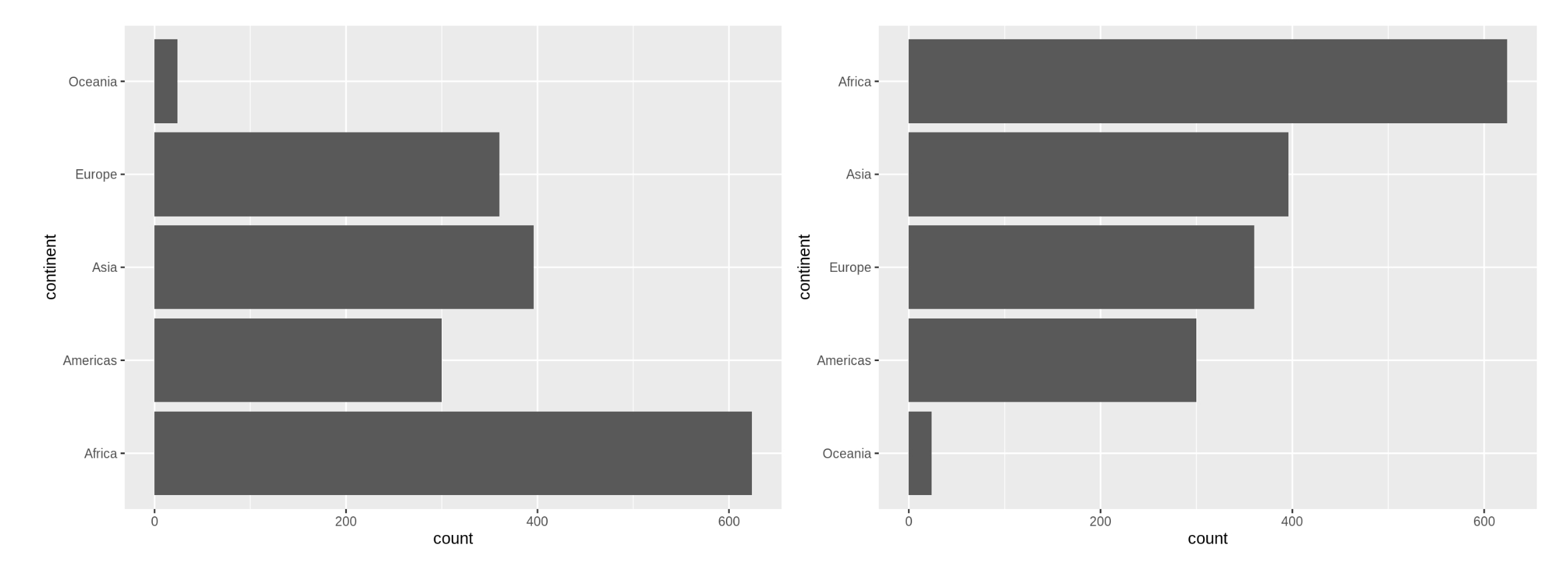
• Factor levels impact statistical analysis & data visualization!

• For example, these two barcharts of frequency by continent differ only in the order of the continents. Which do you prefer? Discuss with your neighbour.

What did we learn today?

• The differences between data frames and tibbles

• The beautiful {lubridate} package for working with dates and times

• Tools for manipulating and working with character data in the {stringr} and {tidyr} packages

• How to take control of our factors using {forcats} and how to investigate factors using base R functions

Attributions

• Stat 545 created by Jenny Bryan

• R for Data Science by Garrett Grolemund & Hadley Wickham