Lecture 4 - Combinging data frames (binds and joins) & base R control flow

Lecture learning objectives:

By the end of this lecture and worksheet 4, students should be able to:

• Compare and contrast mutating joins, filtering joins and set operations

• Choose the appropriate two table dplyr function based on the type of join desired between two data frames, and use it in R to obtained the desired data frame from joining two tables

• Write conditional statements in R with if, else if and else to run different code depending on the input

• Write for loops in R to repeatedly run code

library(tidyverse)
library(gapminder)
options(repr.matrix.max.rows = 10)

Error in library(tidyverse): there is no package called ‘tidyverse’
Traceback:

1. library(tidyverse)

Combining two data tables

We will talk about two different ways of combining data tables in R:

• binds

• joins

Binds

This is basically smashing rocks tibbles together. You can smash things together row-wise (“row binding”) or column-wise (“column binding”).

Why do I characterize this as rock-smashing? They’re often fairly crude operations, with lots of responsibility falling on the analyst for making sure that the whole enterprise even makes sense.

Row binding

When row binding, you need to consider the variables in the two tibbles. Do the same variables exist in each? Are they of the same type? Different approaches for row binding have different combinations of flexibility vs rigidity around these matters.

Let’s bind 3 data frames together vertically (row binding):

fship <- tribble(
                         ~Film,    ~Race, ~Female, ~Male,
  "The Fellowship Of The Ring",    "Elf",    1229,   971,
  "The Fellowship Of The Ring", "Hobbit",      14,  3644,
  "The Fellowship Of The Ring",    "Man",       0,  1995
)
rking <- tribble(
                         ~Film,    ~Race, ~Female, ~Male,
      "The Return Of The King",    "Elf",     183,   510,
      "The Return Of The King", "Hobbit",       2,  2673,
      "The Return Of The King",    "Man",     268,  2459
)
ttow <- tribble(
                         ~Film,    ~Race, ~Female, ~Male,
              "The Two Towers",    "Elf",     331,   513,
              "The Two Towers", "Hobbit",       0,  2463,
              "The Two Towers",    "Man",     401,  3589
)
fship
rking
ttow

A tibble: 3 × 4

Film	Race	Female	Male
<chr>	<chr>	<dbl>	<dbl>
The Fellowship Of The Ring	Elf	1229	971
The Fellowship Of The Ring	Hobbit	14	3644
The Fellowship Of The Ring	Man	0	1995

A tibble: 3 × 4

Film	Race	Female	Male
<chr>	<chr>	<dbl>	<dbl>
The Return Of The King	Elf	183	510
The Return Of The King	Hobbit	2	2673
The Return Of The King	Man	268	2459

A tibble: 3 × 4

Film	Race	Female	Male
<chr>	<chr>	<dbl>	<dbl>
The Two Towers	Elf	331	513
The Two Towers	Hobbit	0	2463
The Two Towers	Man	401	3589

tribble is another function that you can use to make tibbles, but let’s you write the data in a more human readable form.

# bind the rows
bind_rows(fship, ttow, rking)

A tibble: 9 × 4

Film	Race	Female	Male
<chr>	<chr>	<dbl>	<dbl>
The Fellowship Of The Ring	Elf	1229	971
The Fellowship Of The Ring	Hobbit	14	3644
The Fellowship Of The Ring	Man	0	1995
The Two Towers	Elf	331	513
The Two Towers	Hobbit	0	2463
The Two Towers	Man	401	3589
The Return Of The King	Elf	183	510
The Return Of The King	Hobbit	2	2673
The Return Of The King	Man	268	2459

Column binding

When column binding, the onus is entirely on the analyst to make sure that the rows are aligned. I would avoid column binding whenever possible. If you can introduce new variables through any other, safer means, do so! By safer, I mean: use a mechanism where the row alignment is correct by definition. A proper join is the gold standard. In addition to joins, functions like dplyr::mutate() and tidyr::separate() can be very useful for forcing yourself to work inside the constraint of a tibble.

Let’s bind 3 columns onto a data frame:

fship <- tribble(
                         ~Film,    
  "The Fellowship Of The Ring",
  "The Fellowship Of The Ring", 
  "The Fellowship Of The Ring"
)

fship_data <- tribble(
  ~Race, ~Female, ~Male,
  "Elf",    1229,   971,
  "Hobbit",      14,  3644,
  "Man",       0,  1995
)

fship
fship_data

A tibble: 3 × 1

Film
<chr>
The Fellowship Of The Ring
The Fellowship Of The Ring
The Fellowship Of The Ring

A tibble: 3 × 3

Race	Female	Male
<chr>	<dbl>	<dbl>
Elf	1229	971
Hobbit	14	3644
Man	0	1995

# bind the columns
bind_cols(fship, fship_data)

A tibble: 3 × 4

Film	Race	Female	Male
<chr>	<chr>	<dbl>	<dbl>
The Fellowship Of The Ring	Elf	1229	971
The Fellowship Of The Ring	Hobbit	14	3644
The Fellowship Of The Ring	Man	0	1995

Joins

Here you designate a variable (or a combination of variables) as a key. A row in one data frame gets matched with a row in another data frame because they have the same key. You can then bring information from variables in a secondary data frame into a primary data frame based on this key-based lookup. That description is incredibly oversimplified, but that’s the basic idea.

A variety of row- and column-wise operations fit into this framework, which implies there are many different flavors of join. The concepts and vocabulary around joins come from the database world. The relevant functions in dplyr follow this convention and all mention join.

Your best cheatsheet: https://stat545.com/join-cheatsheet.html

Compliments of Jenny Bryan!

Left join

left_join(x, y): Return all rows from x, and all columns from x and y. If there are multiple matches between x and y, all combination of the matches are returned. This is a mutating join.

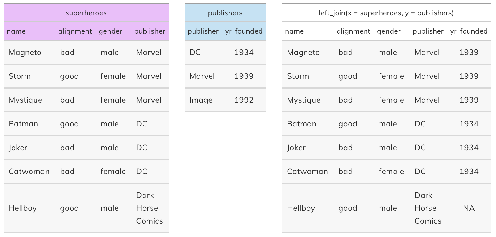
Source: https://stat545.com/join-cheatsheet.html

Let’s work through an example. We will create a data frame called am_af_countries from American and African countries from the gapminder data set, that contains the country and continent rows:

am_af_countries <- gapminder %>% 
    filter(continent == "Americas" | continent == "Africa") %>% 
    select(country, continent) %>% 
    group_by(country) %>% 
    slice(1)
am_af_countries

A grouped_df: 77 × 2

country	continent
<fct>	<fct>
Algeria	Africa
Angola	Africa
Argentina	Americas
Benin	Africa
Bolivia	Americas
⋮	⋮
United States	Americas
Uruguay	Americas
Venezuela	Americas
Zambia	Africa
Zimbabwe	Africa

country_codes

A tibble: 187 × 3

country	iso_alpha	iso_num
<chr>	<chr>	<int>
Afghanistan	AFG	4
Albania	ALB	8
Algeria	DZA	12
Angola	AGO	24
Argentina	ARG	32
⋮	⋮	⋮
Vietnam	VNM	704
West Bank and Gaza	PSE	275
Yemen, Rep.	YEM	887
Zambia	ZMB	894
Zimbabwe	ZWE	716

# join data frames
left_join(am_af_countries, country_codes) 

Joining, by = "country"

A grouped_df: 77 × 4

country	continent	iso_alpha	iso_num
<chr>	<fct>	<chr>	<int>
Algeria	Africa	DZA	12
Angola	Africa	AGO	24
Argentina	Americas	ARG	32
Benin	Africa	BEN	204
Bolivia	Americas	BOL	68
⋮	⋮	⋮	⋮
United States	Americas	USA	840
Uruguay	Americas	URY	858
Venezuela	Americas	VEN	862
Zambia	Africa	ZMB	894
Zimbabwe	Africa	ZWE	716

What if your column names don’t match?

You can specify which columns to join by!

#rename country column _renamed <- am_af_countries %>% 
am_af_countries <- am_af_countries %>% 
    rename(countries = country)
am_af_countries

A grouped_df: 77 × 2

countries	continent
<fct>	<fct>
Algeria	Africa
Angola	Africa
Argentina	Americas
Benin	Africa
Bolivia	Americas
⋮	⋮
United States	Americas
Uruguay	Americas
Venezuela	Americas
Zambia	Africa
Zimbabwe	Africa

left_join(am_af_countries, country_codes, 
          by = c("countries" = "country"))

A grouped_df: 77 × 4

countries	continent	iso_alpha	iso_num
<chr>	<fct>	<chr>	<int>
Algeria	Africa	DZA	12
Angola	Africa	AGO	24
Argentina	Americas	ARG	32
Benin	Africa	BEN	204
Bolivia	Americas	BOL	68
⋮	⋮	⋮	⋮
United States	Americas	USA	840
Uruguay	Americas	URY	858
Venezuela	Americas	VEN	862
Zambia	Africa	ZMB	894
Zimbabwe	Africa	ZWE	716

Other joins:

There are several other joins available to you in the {dplyr} package. I give a high level overview next, and then you will get a chance to interact and explore these functions in more detail in your worksheet and lab.

Inner join

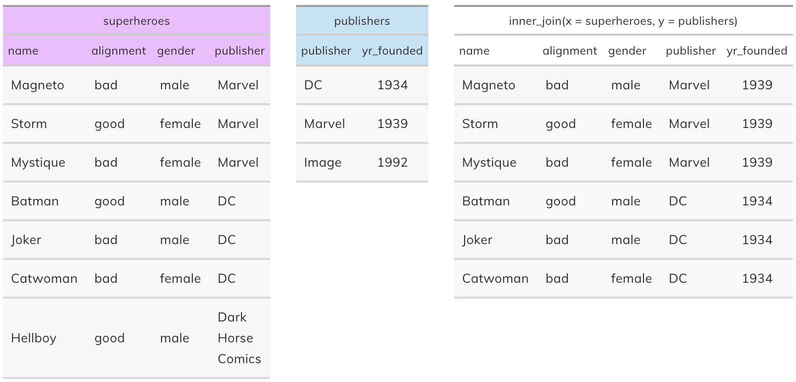
inner_join(x, y): Return all rows from x where there are matching values in y, and all columns from x and y. If there are multiple matches between x and y, all combination of the matches are returned. This is a mutating join.

Source: https://stat545.com/join-cheatsheet.html

Semi join

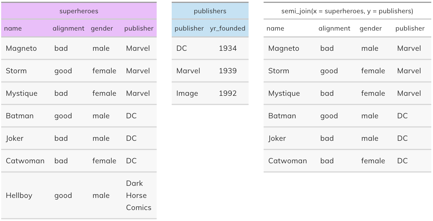
semi_join(x, y): Return all rows from x where there are matching values in y, keeping just columns from x. A semi join differs from an inner join because an inner join will return one row of x for each matching row of y, where a semi join will never duplicate rows of x. This is a filtering join.

Source: https://stat545.com/join-cheatsheet.html

Anti join

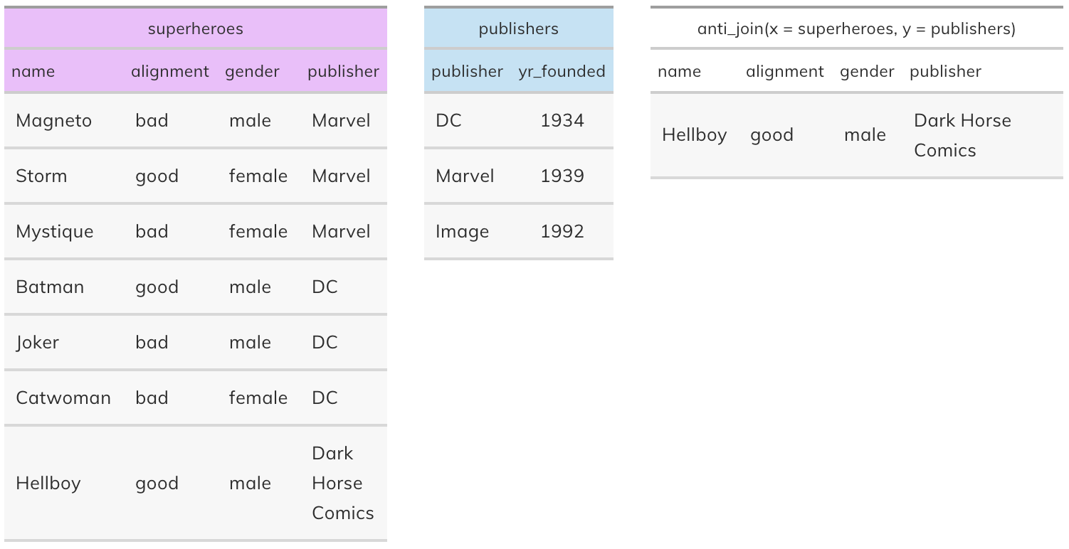
anti_join(x, y): Return all rows from x where there are not matching values in y, keeping just columns from x. This is a filtering join.

Source: https://stat545.com/join-cheatsheet.html

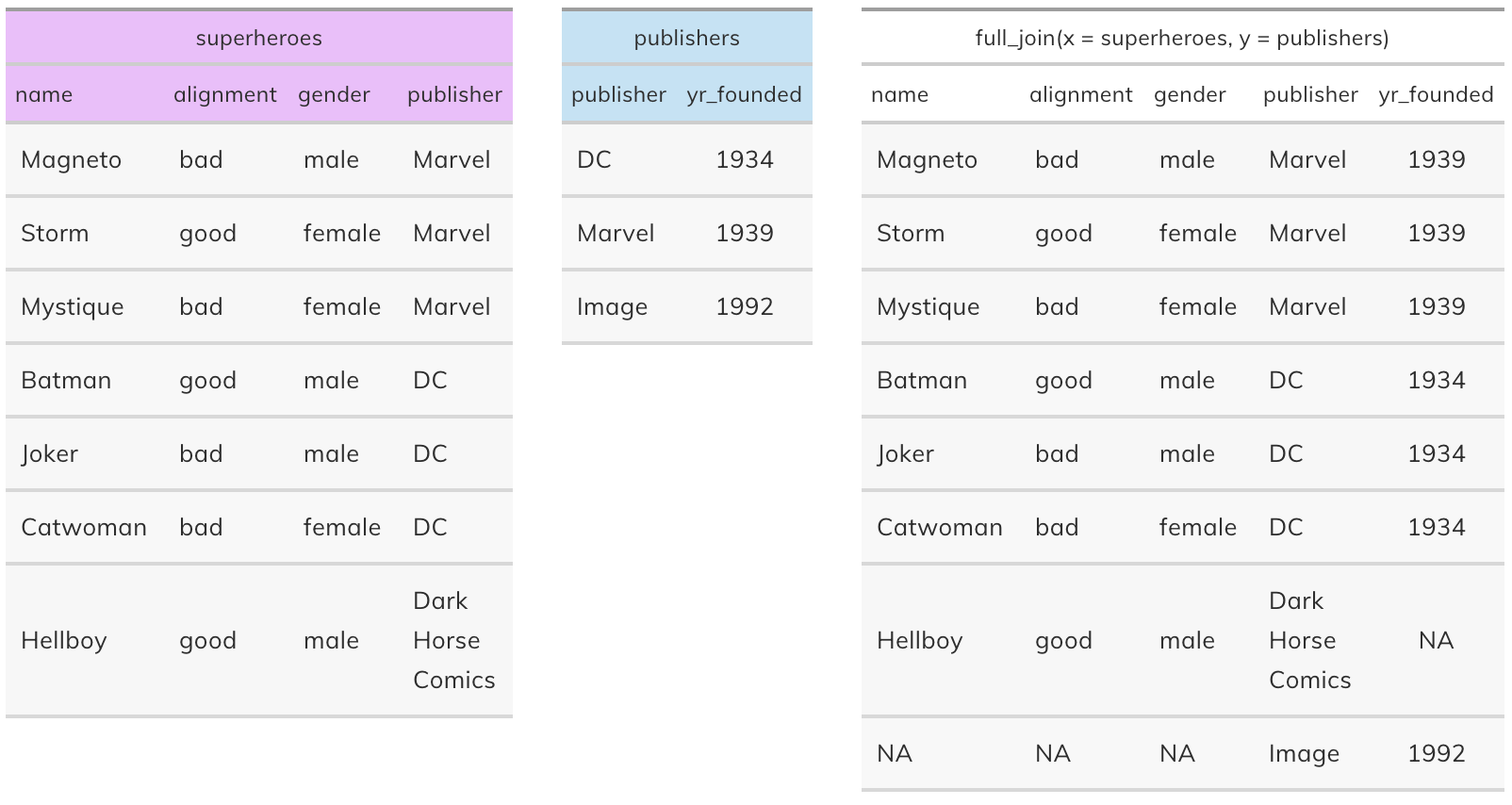
Full join

full_join(x, y): Return all rows and all columns from both x and y. Where there are not matching values, returns NA for the one missing. This is a mutating join.

Source: https://stat545.com/join-cheatsheet.html

Control flow in base R

Similar to other programming languages, R has the now standard control flow capabilities. We will talk about two in this course:

• for loops

• if / else if / else statements (conditionals)

Control Flow: for loops

• For loops in R, work like this: for (item in vector) perform_action

• When code needs to be split across lines in R, we use the { operator to surround it

Iterating over an object

Let’s write a for loop that iterates over a vector of the numbers 1, 2, 3 and prints out the square of each.

sequence <- c(2, 3, 4)
sequence
typeof(sequence)

1. 2
2. 3
3. 4

'double'

for (number in sequence) {
    print(number ^ 2)
}

[1] 4
[1] 9
[1] 16

Using indices in a for loop

for (i in seq_along(sequence)) {
    print(sequence[i] ^ 2)
}

[1] 4
[1] 9
[1] 16

Why use seq_along?

It gives you a sequence along the item you want to iterate over.

seq_along(sequence)

1. 1
2. 2
3. 3

Beware of using length instead:

sequence <- c()
for (i in seq_along(sequence)) {
    print(sequence[i]^2)
    print(i)
}

There is nothing in the vector! Nothing should be printed!

Source: Advanced R by Hadley Wickham

Control Flow: if, if else and else statements

The basic form of an if statement in R is as follows:

if (condition) true_action

if (condition) true_action else false_action

• Again, when code needs to be split across lines in R, we use the { operator to surround it to create code blocks

Example

Below we write a conditional which compares a threshold with a measure. It prints “Over the limit” if the measure is over the threshold, “Under the limit” if the measure is under the threshold and “Exactly at threshold” otherwise.

threshold <- 95.0
measure  <- 93.5

if (measure > threshold) {
    print("Over the limit")
} else if (measure < threshold) {
    print("Under the limit")
} else {
    print("Exactly at threshold")
}

[1] "Under the limit"

Notes - you do not have to use else if, or even else if it doesn’t make sense. I just wanted to demonstrate the full control flow syntax. Additionally, you can have multiple else if statements if you have > 3 choices to make.

Attributions

• Stat 545 created by Jenny Bryan

• R for Data Science by Garrett Grolemund & Hadley Wickham