Lecture 6: Functions and testing in R#

Note from Firas

Our series of R lectures will be presented by Dr. Tiffany Timbers, the other option co-director of the Vancouver MDS program.

Correction from last class:#

You can do manipulations across rows as well as columns in R with data frames without iteration:

head(cars)

A data.frame: 6 × 2
	speed	dist
	<dbl>	<dbl>
1	4	2
2	4	10
3	7	4
4	7	22
5	8	16
6	9	10

cars[1:3, ] <- (cars[1:3, ] + 1)
head(cars)

A data.frame: 6 × 2
	speed	dist
	<dbl>	<dbl>
1	5	3
2	5	11
3	8	5
4	7	22
5	8	16
6	9	10

The memory implications I stated on Tuesday however, still stand.

Another question from lab#

What is a factor?

df <- data.frame(province = c("BC", "AB", "ON"), location = c("west", "west", "east"))
df

A data.frame: 3 × 2
province	location
<chr>	<chr>
BC	west
AB	west
ON	east

str(df)

'data.frame':	3 obs. of  2 variables:
 $ province: chr  "BC" "AB" "ON"
 $ location: chr  "west" "west" "east"

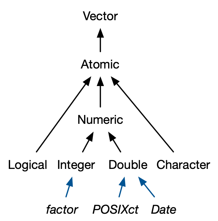
Factors are integer vectors with attributes#

have two attributes:
- class
- levels

typeof(df$location)

'character'

attributes(df$location)

NULL

used to store categorical data, and very useful for data visualization and modeling
not at all helpful for data wrangling

Other vector types built on top of the atomic vectors#

https://d33wubrfki0l68.cloudfront.net/baa19d0ebf9b97949a7ad259b29a1c4ae031c8e2/8e9b8/diagrams/vectors/summary-tree-s3-1.png

Writing readable R code#

WriTing AND reading (code) TaKes cognitive RESOURCES, & We only hAvE so MUCh!
To help free up cognitive capacity, we will follow the tidyverse style guide

Sample code not in tidyverse style#

Can we spot what’s wrong?

Sample code in tidyverse style#

Lecture learning objectives:#

By then end of the lecture & lab 3, students should be able to:

In R, define and use a named function that accepts parameters and returns values
Describe lazy evaluation and ... (variable arguments) and how it affects functions in R
explain the importance of scoping and environments in R as they relate to functions
Use testthat to formulate a test case to prove a function design specification
Use test-driven development principles to define a function that accepts parameters, returns values and passes all tests

Handle errors gracefully via exception handling
Use roxygen2 friendly function documentation to describe parameters, return values, description and example(s).
Write comments within a function to improve readability
Evaluate the readability, complexity and performance of a function
Source and use functions stored as R code in another file, as well as those in R packages/libraries
Describe what R packages/libraries are, as well as explain when and why they are useful

Defining functions in R#

Use variable <- function(…arguments…) { …body… } to create a function and give it a name

Example:

add <- function(x, y) {
  x + y
}

add(5, 10)

As in Python, functions in R are objects. This is referred to as “first-class functions”.
The last line of the function returns a value, to return a value early use the special word return

add <- function(x, y) {
    if (!is.numeric(x) | !is.numeric(y)) {
        return(NA)
    }
    x + y
}

add(5, "a")

<NA>

Note: you probably want to throw an error here instead of return NA, this example was purely for illustrating early returns

Default function arguments#

Same as in Python!

repeat_string <- function(x, n = 2) {
    repeated <- ""
    for (i in seq_along(1:n)) {
        repeated <- paste0(repeated, x)
    }
    repeated
}

repeat_string("MDS")

'MDSMDS'

Optional - Advanced#

Extra arguments via `...`#

If we want our function to be able to take extra arguments that we don’t specify, we must explicitly convert ... to a list:

add <- function(x, y, ...) {
    total = x + y
    for (value in list(...)) {
        total <- total + value
    }
    total
    print(list(...))
}
add(1, 3, 5, 6)

[[1]]
[1] 5

[[2]]
[1] 6

Lexical scoping in R#

R’s lexical scoping follows several rules, we will cover the following 3:

Name masking
Dynamic lookup
A fresh start

Name masking#

Names defined inside a function mask names defined outside a function

If a name isn’t defined inside a function, R looks one level up (and then all the way up into the global environment and even loaded packages!)

Talk through the following code with your neighbour and predict the output, then let’s confirm the result by running the code.

x <- 1
g04 <- function() {
  y <- 2
  i <- function() {
    z <- 3
    c(x, y, z)
  }
  i()
}
g04()

Dynamic lookup#

R looks for values when the function is run, not when the function is created.
This means that the output of a function can differ depending on the objects outside the function’s environment.

Talk through the following code with your neighbour and predict the output, then let’s confirm the result by running the code.

g12 <- function() x + 1
x <- 15
g12()

x <- 20
g12()

A fresh start#

Every time a function is called a new environment is created to host its execution.
This means that a function has no way to tell what happened the last time it was run; each invocation is completely independent.

Talk through the following code with your neighbour and predict the output, then let’s confirm the result by running the code.

g11 <- function() {
  if (!exists("a")) {
    a <- 1
  } else {
    a <- a + 1
  }
  a
}

g11()
g11()
g11()

Lazy evaluation#

In R, function arguments are lazily evaluated: they’re only evaluated if accessed.

Knowing that, now consider the add_one function written in both R and Python below:

# R code (this would work)
add_one <- function(x, y) {
    x <- x + 1
    return(x)
} 

# Python code (this would not work)
def add_one(x, y):
    x = x + 1
    return x

Answer the poll on Slack.

Poll:

From the list below, select the reason why the above add_one function will work in R, but the equivalent version of the function in python would break.

Python evaluates the function arguments before it evaluates the function and because it doesn’t know what y is, it will break even though it is not used in the function.
R performs lazy evaluation, meaning it delays the evaluation of the function arguments until its value is needed within/inside the function.
The question is wrong, both functions would work in their respective languages.
answer 1 & 2 are correct

The power of lazy evaluation#

Let’s you have easy to use interactive code like this:

head(mtcars, n = 2)

A data.frame: 2 × 11
	mpg	cyl	disp	hp	drat	wt	qsec	vs	am	gear	carb
	<dbl>	<dbl>	<dbl>	<dbl>	<dbl>	<dbl>	<dbl>	<dbl>	<dbl>	<dbl>	<dbl>
Mazda RX4	21	6	160	110	3.9	2.620	16.46	0	1	4	4
Mazda RX4 Wag	21	6	160	110	3.9	2.875	17.02	0	1	4	4

dplyr::select(mtcars, mpg, cyl, hp, qsec)

Error in loadNamespace(x): there is no package called ‘dplyr’
Traceback:

1. loadNamespace(x)
2. withRestarts(stop(cond), retry_loadNamespace = function() NULL)
3. withOneRestart(expr, restarts[[1L]])
4. doWithOneRestart(return(expr), restart)

Notes:

There’s more than just lazy evaluation happening in the code above, but lazy evaluation is part of it.
package::function() is a way to use a function from an R package without loading the entire library.

Function composition#

You have 3 options in R:

assigning values to intermediate objects,
nested function calls, or
the binary operator %>%, which is called the pipe and is pronounced as “and then”.

For example, imagine you want to compute the population standard deviation using sqrt() and mean() as building blocks, and we create the two functions:

square <- function(x) {
    x^2
}
deviation <- function(x) {
    x - mean(x)
}
x <- runif(100)
x

Option 1: assigning values to intermediate objects

out <- deviation(x)
out <- square(out)
out <- mean(out)
out <- sqrt(out)
out

Option 2: nested function calls

sqrt(mean(square(deviation(x))))

Option 3: the binary operator %>%, which is called the pipe and is pronounced as “and then”.

library(magrittr, quietly = TRUE) # also loaded as a dependency of dplyr and tidyverse

x %>%
  deviation() %>%
  square() %>%
  mean() %>%
  sqrt()

What to choose?#

Each of the three options has its own strengths and weaknesses:

Intermediate objects:

requires you to name intermediate objects. This is a strength when objects are important, but a weakness when values are truly intermediate.

Nesting:

is concise, and well suited for short sequences.
But longer sequences are hard to read because they are read inside out and right to left.

Piping:

allows you to read code in straightforward left-to-right fashion and doesn’t require you to name intermediate objects.
But you can only use it with linear sequences of transformations of a single object.
It also requires an additional third party package and assumes that the reader understands piping.

5 min break#

Writing tests in R with test_that#

Industry standard tool for writing tests in R is the testthat package.
To use an R package, we typically load the package into R using the library function:

library(testthat)

How to write a test with `testthat::test_that`#

test_that("Message to print if test fails", expect_*(...))

Often our test_that function calls are longer than 80 characters, so we use { to split the code across multiple lines, for example:

x <- c(3.5, 3.5, 3.5)
y <- c(3.5, 3.5, 3.49999)
test_that("x and y should contain the same values", {
    expect_equal(x, y)
})

Are you starting to see a pattern with { yet…

Common `expect_*` statements for use with `test_that`#

Is the object equal to a value?#

expect_identical - test two objects for being exactly equal
expect_equal - compare R objects x and y testing ‘near equality’ (can set a tolerance)
expect_equivalent - compare R objects x and y testing ‘near equality’ (can set a tolerance) and does not assess attributes

Does code produce an output/message/warning/error?#

expect_error - tests if an expression throws an error
expect_warning - tests whether an expression outputs a warning
expect_output - tests that print output matches a specified value

Is the object true/false?#

These are fall-back expectations that you can use when none of the other more specific expectations apply. The disadvantage is that you may get a less informative error message.

expect_true - tests if the object returns TRUE
expect_false - tests if the object returns FALSE

Challenge 1:#

Add a tolerance arguement to the expect_equal statement such that the observed difference between these very similar vectors doesn’t cause the test to fail.

x <- c(3.5, 3.5, 3.5)
y <- c(3.5, 3.5, 3.49999)
test_that("x and y should contain the same values", {
    expect_equal(x, y)
})

Unit test example#

celsius_to_fahr <- function(temp) {
  (temp * (9 / 5)) + 32
}

test_that("Temperature should be the same in Celcius and Fahrenheit at -40", {
        expect_identical(celsius_to_fahr(-40), -40)
    })
test_that("Room temperature should be about 23 degrees in Celcius and 73 degrees Fahrenheit", {
        expect_equal(celsius_to_fahr(23), 73, tolerance = 1)
    })

Test-driven development (TDD) review#

Write your tests first (that call the function you haven’t yet written), based on edge cases you expect or can calculate by hand
If necessary, create some “helper” data to test your function with (this might be done in conjunction with step 1)
Write your function to make the tests pass (in this process you might think of more tests that you want to add)

Toy example of how TDD can be helpful#

Let’s create a function called fahr_to_celsius that converts temperatures from Fahrenheit to Celsius.

First we’ll write the tests (which will fail):

test_fahr_to_celsius <- function() {
    test_that("Temperature should be the same in Celcius and Fahrenheit at -40", {
        expect_identical(fahr_to_celsius(-40), -40)
    })
    test_that("Room temperature should be about 73 degrees Fahrenheit and 23 degrees in Celcius", {
        expect_equal(fahr_to_celsius(73), 23, tolerance = 1)
    })
}

Then we write our function to pass the tests:

fahr_to_celsius <- function(temp) {
    (temp + 32) * 5/9
}

Then we call our tests to check it:

test_fahr_to_celsius()

Exception handling in R#

How to check type and throw an error if not the expected type:

if (!is.numeric(c(1, 2, "c")))
  stop("Cannot compute of a vector of characters.")

Example of defensive programming at the beginning of a function:

fahr_to_celsius <- function(temp) {
    if(!is.numeric(temp)){
        stop("Cannot calculate temperature in Farenheit for non-numerical values")
    }
    (temp - 32) * 5/9
}

fahr_to_celsius("thirty")

If you wanted to issue a warning instead of an error, you could use warning in place of stop in the example above. However, in most cases it is better practice to throw an error than to print a warning…

We can test our exceptions using test_that:#

test_that("Non-numeric values for temp should throw an error", {
    expect_error(fahr_to_celsius("thirty"))
    expect_error(fahr_to_celsius(list(4)))
    })

`try` in R#

Similar to Python, R has a try function to attempt to run code, and continue running subsequent code even if code in the try block does not work:

try({
    # some code
    # that can be 
    # split across several
    # lines
})

# code to continue even if error in code 
# in try code block above

This code normally results in an error that stops following code from running:

x <- data.frame(col1 = c(1, 2, 3, 2, 1), 
                col2 = c(0, 1, 0, 0 , 1))
x[3]
dim(x)

Try let’s the code following the error run:

try({x <- data.frame(col1 = c(1, 2, 3, 2, 1), 
                     col2 = c(0, 1, 0, 0 , 1))
     x[3]
})
dim(x)

Sensibly (IMHO) try has a default of silent=FALSE, which you can change if you find good reason too.

`roxygen2` friendly function documentation#

#' Converts temperatures from Fahrenheit to Celsius.
#'    
#' @param temp a vector of temperatures in Fahrenheit
#' 
#' @return a vector of temperatures in Celsius
#' 
#' @examples
#' fahr_to_celcius(-20)
fahr_to_celsius <- function(temp) {
    (temp - 32) * 5/9
}

Why roxygen2 documentation? If you document your functions like this, when you create an R package to share them they will be set up to have the fancy documentation that we get using ?function_name.

RStudio has template for `roxygen2` documentation#

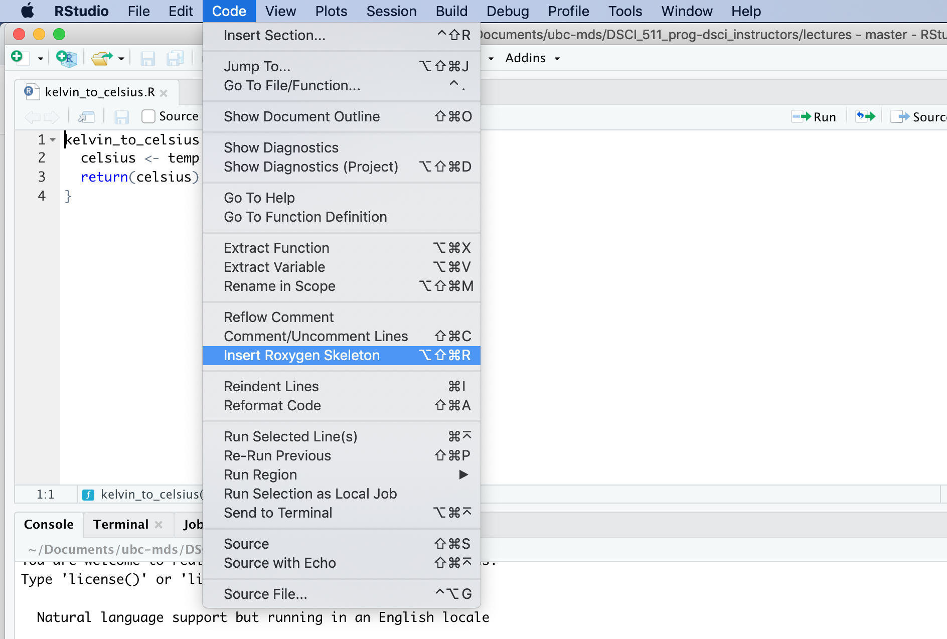
Reading in functions from an R script#

Usually the step before packaging your code, is having some functions in another script that you want to read into your analysis. We use the source function to do this:

source("src/kelvin_to_celsius.R")

Once you do this, you have access to all functions contained within that script:

kelvin_to_celsius(273.15)

Note - this is how the test_* functions are brought into your Jupyter notebooks for the autograding part of your lab3 homework.

Introduction to R packages#

source("script_with_functions.R") is useful, but when you start using these functions in different projects you need to keep copying the script, or having overly specific paths…

The next step is packaging your R code so that it can be installed and then used across multiple projects on your (and others) machines without directly pointing to where the code is stored, but instead accessed using the library function.

You will learn how to do this in Collaborative Software Development (term 2), but for now, let’s tour a simple R package to get a better understanding of what they are: https://github.com/ttimbers/convertemp

Install the convertemp R package:#

In RStudio, type: devtools::install_github("ttimbers/convertemp")

library(convertemp)

?celsius_to_kelvin

celsius_to_kelvin(0)

What did we learn today?#

Attribution:#

Advanced R by Hadley Wickham
The Tidynomicon by Greg Wilson

Data 531

Lecture 6: Functions and testing in R

Contents

Lecture 6: Functions and testing in R#

Correction from last class:#

Another question from lab#

Factors are integer vectors with attributes#

Other vector types built on top of the atomic vectors#

Writing readable R code#

Sample code not in tidyverse style#

Sample code in tidyverse style#

Lecture learning objectives:#

Defining functions in R#

Default function arguments#

Optional - Advanced#

Extra arguments via ...#

Lexical scoping in R#

Name masking#

Dynamic lookup#

A fresh start#

Lazy evaluation#

The power of lazy evaluation#

Function composition#

What to choose?#

5 min break#

Writing tests in R with test_that#

How to write a test with testthat::test_that#

Common expect_* statements for use with test_that#

Is the object equal to a value?#

Does code produce an output/message/warning/error?#

Is the object true/false?#

Challenge 1:#

Unit test example#

Test-driven development (TDD) review#

Toy example of how TDD can be helpful#

Exception handling in R#

We can test our exceptions using test_that:#

try in R#

roxygen2 friendly function documentation#

RStudio has template for roxygen2 documentation#

Reading in functions from an R script#

Introduction to R packages#

Install the convertemp R package:#

What did we learn today?#

Attribution:#

Extra arguments via `...`#

How to write a test with `testthat::test_that`#

Common `expect_*` statements for use with `test_that`#

`try` in R#

`roxygen2` friendly function documentation#

RStudio has template for `roxygen2` documentation#