551 Lec 6 - Linking plots, maps in plotly and deployment on Heroku
You need to download this notebook to view images.
Lecture learning goals
By the end of the lecture you will be able to:
Implement server side interactivity between plots
Work with geojson files in plotly
Create maps with interactivity
Setup and Heroku account and run the Heroku CLI
Prepare the necessary files for deployment
Push to Heroku’s repo and troubleshoot remote errors
Linking interactive plots
What is the return value from the selected data in a scatter plot?
Let’s start from where we left off last lecture.
library(dash)
library(dashCoreComponents)
library(dashHtmlComponents)
library(dashBootstrapComponents)
library(ggplot2)
library(plotly)
app <- Dash$new(external_stylesheets = dbcThemes$BOOTSTRAP)
app$layout(
dbcContainer(
list(
dccGraph(id='plot-area'),
htmlDiv(id='output-area'),
htmlBr(),
dccDropdown(
id='col-select',
options = msleep %>% colnames %>% purrr::map(function(col) list(label = col, value = col)),
value='bodywt')
)
)
)
app$callback(
output('plot-area', 'figure'),
list(input('col-select', 'value')),
function(xcol) {
p <- ggplot(msleep) +
aes(x = !!sym(xcol),
y = sleep_total,
color = vore,
text = name) +
geom_point() +
scale_x_log10() +
ggthemes::scale_color_tableau()
ggplotly(p, tooltip = 'text') %>% layout(dragmode = 'select')
}
)
app$callback(
output('output-area', 'children'),
list(input('plot-area', 'selectedData')),
function(selected_data) {
list(toString(selected_data))
}
)
app$run_server(debug = T)
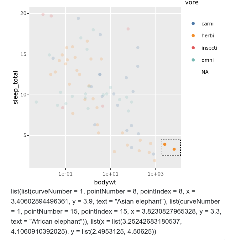
The output from our selected data look like this when displayed as a string in the HTML div.
Another way to see these lists of names lists is to print them to the console inside your function with print(), and then they will look slightly different.
list(list(curveNumber = 1, pointNumber = 8, pointIndex = 8, x = 3.40602894496361, y = 3.9, text = "Asian elephant"), list(curveNumber = 1, pointNumber = 15, pointIndex = 15, x = 3.8230827965328, y = 3.3, text = "African elephant")), list(x = list(3.25242683180537, 4.1060910392025), y = list(2.4953125, 4.50625))
This is a list consisting of two named lists.
The first one (selected_data[[2]]) is pretty uninteresting for us
as it contains the x and y values of the rectangular selection
we created when dragging with the mouse:
list(x = list(3.25242683180537, 4.1060910392025), y = list(2.4953125, 4.50625))
The first one (selected_data[[1]]) has all the info of our selected points:
list(curveNumber = 1, pointNumber = 8, pointIndex = 8, x = 3.40602894496361, y = 3.9, text = "Asian elephant"),
list(curveNumber = 1, pointNumber = 15, pointIndex = 15, x = 3.8230827965328, y = 3.3, text = "African elephant")
One named list for the first point (Asian elephant) and one for the second point (African elephant).
curveNumberindicates which group/color the point belongs to.pointNumberandpointIndexunfortunately does not represent the row numbers in the data frame, but rather some ordering internal to plotly.The
xandyvalues represent the position of the point in our graph based on the x and y columns we chose.The
textvalue holds everything contained in our tooltip and if we include more than one value, the values will be separated by<br>in the returned string.
The most interesting values for us here are x, y, and text
since these can include features that are useful for filtering data in another callback.
If the feature you want to use for filtering is not on x or y,
include it in the tooltip, ideally as a single value.
Plotly does support a customdata attribute
which can be used to bass along arbitrary features
that you might want to filter on,
but for some reason this does not seem to work with ggplotly.
If you happen to be already using plotly directly for some part of your dashboard,
feel free to use customdata,
but for ggplotly use the strategy outlined above.
How to filter a dataframe based on the selected value
Now that we know which part of the selection we want,
how do we use it to filter our data?
First we need to extract just the part that we want from the named list.
For a single named list,
we could simply access that element with a name,
but since we might select multiple points
we need to map the name access to each point in the list.
In Python this would be a list comprehension,
and in R we can use purrr to map a selection to every item in the list
(similar to what we saw in setting the options for the dropdown)
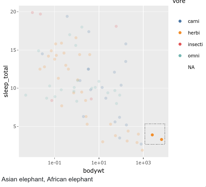
In this example,
we want to grab the text field from the returned selected_data value:
selected_data[[1]] %>% purrr::map_chr('text')
## Asian elephant, African elephant
The return value is a vector of the type we specified in purrr.
If we wanted to grab an integer or float/double instead of a text string,
we would use map_int or map_dbl instead.
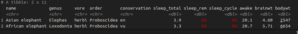
Now that we have these values, we can use them to filter our data frame with like so:
animal_names <- selected_data[[1]] %>% purrr::map_chr('text')
msleep %>% filter(name %in% animal_names)
If you don’t have a unique feature (like name here) to use for filtering,
you can create a “metadata/ID” column consisting of your dataframes rownames
and then assign this to the text and tooltip property,
so that you can use it to reference back to your dataframe.
With these changes, the calback would look like this:
app$callback(
output('output-area', 'children'),
list(input('plot-area', 'selectedData')),
function(selected_data) {
animal_names <- selected_data[[1]] %>% purrr::map_chr('text')
print(msleep %>% filter(name %in% animal_names))
toString(animal_names) # Only for printing the names in the div
}
)
You can see in the printed console output that we have filtered correctly
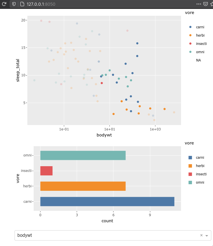
Plotting the selected data via another callback (a.k.a. server side interactivity)
To use these selected values to create a plot, we would set up a regular callback, “purrr out” the values we want, filter our dataframe and use thie data for plotting. We will also change the div output area for another plotting area, so that our app now looks like this:
library(dash)
library(dashCoreComponents)
library(dashHtmlComponents)
library(dashBootstrapComponents)
library(ggplot2)
library(plotly)
app <- Dash$new(external_stylesheets = dbcThemes$BOOTSTRAP)
app$layout(
dbcContainer(
list(
dccGraph(id='plot-area'),
dccGraph(id='bar-plot'),
htmlBr(),
dccDropdown(
id='col-select',
options = msleep %>% colnames %>% purrr::map(function(col) list(label = col, value = col)),
value='bodywt')
)
)
)
app$callback(
output('plot-area', 'figure'),
list(input('col-select', 'value')),
function(xcol) {
p <- ggplot(msleep) +
aes(x = !!sym(xcol),
y = sleep_total,
color = vore,
text = name) +
geom_point() +
scale_x_log10() +
ggthemes::scale_color_tableau()
ggplotly(p, tooltip = 'text') %>% layout(dragmode = 'select')
}
)
app$callback(
output('bar-plot', 'figure'),
list(input('plot-area', 'selectedData')),
function(selected_data) {
animal_names <- selected_data[[1]] %>% purrr::map_chr('text')
p <- ggplot(msleep %>% filter(name %in% animal_names)) +
aes(y = vore,
fill = vore) +
geom_bar(width = 0.6) +
ggthemes::scale_fill_tableau()
ggplotly(p, tooltip = 'text') %>% layout(dragmode = 'select')
}
)
app$run_server(debug = T)
More on ggplotly can be found in the docs and also [in this separate resource, which goes some additional plotly functions we can use to control the ggplot objects)[https://plotly-r.com/improving-ggplotly.html].
Creating maps with plotly
There are a few different approaches to maps we could could we dashr,
including geom_df and leaflet,
and here we will use plotly’s map plotting functions.
We can use our own geojson files with plotly,
and just like for Altair,
they also supply data sets for the coutries of the world,
and the US states.
In fact,
the default in plotly’s choropleth function is to show a map of the world.
df <- read.csv("https://raw.githubusercontent.com/plotly/datasets/master/2014_world_gdp_with_codes.csv")
head(df)
| COUNTRY | GDP..BILLIONS. | CODE | |
|---|---|---|---|
| <chr> | <dbl> | <chr> | |
| 1 | Afghanistan | 21.71 | AFG |
| 2 | Albania | 13.40 | ALB |
| 3 | Algeria | 227.80 | DZA |
| 4 | American Samoa | 0.75 | ASM |
| 5 | Andorra | 4.80 | AND |
| 6 | Angola | 131.40 | AGO |
library(plotly)
plot_ly(df, type='choropleth')
Error in library(plotly): there is no package called ‘plotly’
Traceback:
1. library(plotly)
These are zoomable by default and can be linked to datasets with country codes.
Plotly uses ~ to reference a variable/column name in the dataframe.
plot_ly(df, type='choropleth', locations=~CODE, z=~GDP..BILLIONS.)
The value and country code is shown by default in the tooltip, and we can add any info from the data frame that we want. We can also change the colorscale, either manually as per the docs or to one of these built-in strings:
Greys,YlGnBu,Greens,YlOrRd,Bluered,RdBu,Reds,Blues,Picnic,
Rainbow,Portland,Jet,Hot,Blackbody,Earth,Electric,Viridis,Cividis
plot_ly(df, type='choropleth', locations=~CODE, z=~GDP..BILLIONS., text=~COUNTRY, colorscale='Blues')
Let’s use some US export data to see how we can zoom in on an area of the map.
df <- read.csv("https://raw.githubusercontent.com/plotly/datasets/master/2011_us_ag_exports.csv")
head(df)
| code | state | category | total.exports | beef | pork | poultry | dairy | fruits.fresh | fruits.proc | total.fruits | veggies.fresh | veggies.proc | total.veggies | corn | wheat | cotton | |
|---|---|---|---|---|---|---|---|---|---|---|---|---|---|---|---|---|---|
| <chr> | <chr> | <chr> | <dbl> | <dbl> | <dbl> | <dbl> | <dbl> | <dbl> | <dbl> | <dbl> | <dbl> | <dbl> | <dbl> | <dbl> | <dbl> | <dbl> | |
| 1 | AL | Alabama | state | 1390.63 | 34.4 | 10.6 | 481.0 | 4.06 | 8.0 | 17.1 | 25.11 | 5.5 | 8.9 | 14.33 | 34.9 | 70.0 | 317.61 |
| 2 | AK | Alaska | state | 13.31 | 0.2 | 0.1 | 0.0 | 0.19 | 0.0 | 0.0 | 0.00 | 0.6 | 1.0 | 1.56 | 0.0 | 0.0 | 0.00 |
| 3 | AZ | Arizona | state | 1463.17 | 71.3 | 17.9 | 0.0 | 105.48 | 19.3 | 41.0 | 60.27 | 147.5 | 239.4 | 386.91 | 7.3 | 48.7 | 423.95 |
| 4 | AR | Arkansas | state | 3586.02 | 53.2 | 29.4 | 562.9 | 3.53 | 2.2 | 4.7 | 6.88 | 4.4 | 7.1 | 11.45 | 69.5 | 114.5 | 665.44 |
| 5 | CA | California | state | 16472.88 | 228.7 | 11.1 | 225.4 | 929.95 | 2791.8 | 5944.6 | 8736.40 | 803.2 | 1303.5 | 2106.79 | 34.6 | 249.3 | 1064.95 |
| 6 | CO | Colorado | state | 1851.33 | 261.4 | 66.0 | 14.0 | 71.94 | 5.7 | 12.2 | 17.99 | 45.1 | 73.2 | 118.27 | 183.2 | 400.5 | 0.00 |
p <- plot_ly(df, type = 'choropleth', locationmode = 'USA-states',
z = ~total.exports, locations = ~code, color = ~total.exports, colors = 'Purples')
p
p %>% layout(geo = list(scope = 'usa', projection = list(type = 'albers usa')),
title = 'USA exports')
You can select by dragging, or change to select via clicking. If you also want clicks to send a plotly click even to use in another callback, then use 'event+click'. More about click events in the docs
p %>% layout(geo = list(scope = 'usa', projection = list(type = 'albers usa')),
title = 'USA exports', clickmode = 'event+select')
df <- read.csv('https://raw.githubusercontent.com/plotly/datasets/master/2014_us_cities.csv')
head(df)
| name | pop | lat | lon | |
|---|---|---|---|---|
| <chr> | <int> | <dbl> | <dbl> | |
| 1 | New York | 8287238 | 40.73060 | -73.98658 |
| 2 | Los Angeles | 3826423 | 34.05372 | -118.24273 |
| 3 | Chicago | 2705627 | 41.87555 | -87.62442 |
| 4 | Houston | 2129784 | 29.75894 | -95.36770 |
| 5 | Philadelphia | 1539313 | 39.95233 | -75.16379 |
| 6 | Phoenix | 1465114 | 33.44677 | -112.07567 |
Note that you need to use plot_geo when overlaying points with a longitude and latitude.
The syntax is very similar to plot_ly.
plot_geo(df, locationmode = 'USA-states', sizes = c(5, 250)) %>%
layout(geo = list(scope = 'usa', projection = list(type = 'albers usa'))) %>%
add_markers(x = ~lon, y = ~lat, size = ~pop, text = ~name, hoverinfo = 'text')
Warning message:
“`line.width` does not currently support multiple values.”
Warning message:
“`line.width` does not currently support multiple values.”
To color NANs grey for missing countries, see these links (Python, but it will be similar in R).
Deployment on Heroku
I created a repo with a deployed demo R app with all the files mentioned below that you can clone and test deploy for yourself if you wish.
For deployment we’re going to follow the dash documentation,
with a few important changes (detailed below).
The overall process is that we will create new files with the names and content mentioned in the dash docs to our existing project directory.
Therefore you don’t need to do the first two steps telling your to create a new directory and run git init.
Your overall project structure should look similar to the below
and it can be a good idea to keep app.R in the root instead of in src,
unless you are comfortable making changes to the other files
(it might just be changing the last line of the Dockerfile,
but I have not tested it thoroughly).
├── data
│ └── your-data.csv
├── Dockerfile
├── app.R
├── apt-packages
├── dashr-deploy.Rproj
├── heroku.yml
└── init.R
Changes to the dash docs instructions
Change the your last line to
app$run_server(host = '0.0.0.0')when deploying. This is needed for the app to bind correctly to the ports when deployed and removingdebugalso makes it easier to debug if something goes wrong since you will not see the error message otherwise (ironically enough).Change the first line of the
Dockerfileto pull container3.6.3instead of3.6.2.Use
heretogether wit an.Rprojfile in your project root to ensure that paths work when deployed.Use
init.Rfor installing R packages instead of theDockerfile.Change the last lines of
init.Rto the following, and feel free to add any additional packages you might need:# packages go here install.packages(c('dash', 'readr', 'here', 'ggthemes', 'remotes')) remotes::install_github('facultyai/dash-bootstrap-components@r-release')
The R deployment takes aroudn 15 min, which makes it extra annoying if you mistype something or struggle with package installations. Below are a few tips which could help save you time if you struggle with deployment. If things are working fine, you don’t need the section below.
Some heroku tips and tricks
Heroku has a command that allows us to ssh into the server after it is deployed (heroku ps:exec),
but it doesn’t work on containers out of the box unfortunately
(steps for getting it to work here, I haven’t tried).
Instead we have two options:
we can send individual commands with heroko run,
e.g. heroku run ls etc.
However, these also take some time to run and connect each time.
Instead we could once send heroku run bash
which will put us in a bash shell on the server
and allow us to navigate the file system and check installed packages etc.
Of particular notice would be checking which R packages are installed,
via one of these commands:
Rscript -e "installed.packages()[,c('Package', 'Version')]"
# OR
Rscript -e "installed.packages()[,c('Package', 'Version')]" | grep readr
There is no command line text editor installed by default,
so if you want to make small changes to your files,
you would need to follow the steps outlined here to install either vim or nano.
However,
if modify app.R this way,
it will not update even if you have debug = T in app$run_server
(I believe this is because we are in a new shell rather than sshing into the one where our dashboard is actually running).
Also note that all files are removed when you push to heroku,
so don’t make any extensive changes on the dyno itself.
Attribution
These lecture notes were prepared by Dr. Joel Ostblom, a post-doctoral teaching fellow in the UBC Vancouver MDS program.